In This Topic
Method table
The Method table shows the settings for the analysis and the selected lag order.
In these results, the maximum lag order that the analysis evaluates is 9. The analysis uses the model with the highest lag order of 4 to calculate the test results.
Method
| Maximum lag order for terms in the regression model | 9 |
|---|---|
| Criterion for selecting lag order | Minimum AIC |
| Additional terms | Constant |
| Selected lag order | 4 |
| Rows used | 36 |
Augmented Dickey-Fuller Test table
The Augmented Dickey-Fuller Test table provides the hypotheses, a test statistic, a p-value, and a recommendation about whether to consider differencing to make the series stationary.
The test statistic provides one way to evaluate the null hypothesis. Test statistics that are less than or equal to the critical value provide evidence against the null hypothesis.
The p-value is a probability that measures the evidence against the null hypothesis. Lower probabilities provide stronger evidence against the null hypothesis.
To determine whether to difference the data, compare the test statistic to the critical value or the p-value to your significance level. Because the p-value contains more approximation, the recommendation from the analysis uses the critical value to assess the null hypothesis when the significance level is 0.01, 0.05, or 0.10. Usually, the conclusion is the same for the critical value and the p-value. The null hypothesis is that the data are non-stationary, which implies that differencing is a reasonable step to try to make the data stationary.
- P-value ≤ significance level
- Test statistic ≤ critical value
- If the p-value is less than or equal to the significance level or if the test statistic is less than or equal to the critical value, the decision is to reject the null hypothesis. Because the data provide evidence that the data are stationary, the recommendation of the analysis is to proceed without differencing.
- P-value > significance level
- Test statistic > critical value
- If the p-value is greater than the significance level or if the test statistic is greater than the critical value, the decision is to fail to reject the null hypothesis. Because the data do not provide evidence that the data are stationary, the recommendation of the analyis is to determine whether differencing makes the mean of the data stationary.
In these results, the test statistic of 2.29045 is greater than the critical value of approximately -2.96053. Because the results fail to reject the null hypothesis that the data are non-stationary, the recommendation of the test is to consider differencing to make the data stationary.
Augmented Dickey-Fuller Test
| Null hypothesis: | Data are non-stationary |
|---|---|
| Alternative hypothesis: | Data are stationary |
| Test Statistic | P-Value | Recommendation |
|---|---|---|
| 2.29045 | 0.999 | Test statistic > critical value of -2.96053. |
| Significance level = 0.05 | ||
| Fail to reject null hypothesis. | ||
| Consider differencing to make data stationary. |
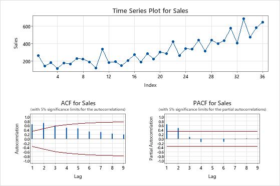
Plots of the original series
- Time series plot
- Use the time series plot of the original series to examine the characteristics of the original data. A trend is an example of a pattern that indicates a non-stationary mean. Use differencing to try to make the mean stationary.
- ACF plot
- Use the autocorrelation function (ACF) from the original data to look for a pattern that indicates that the mean of the data is not stationary. A common pattern is large spikes across lags that die out very slowly.
- PACF plot
- Usually, you use the partial autocorrelation function (PACF) of stationary data to look for patterns that indicate the presence of autoregressive terms in an ARIMA model. If the original data are not stationary, use the PACF plot of the differenced series to look for candidate terms for the ARIMA model.
In these results, the data show an increasing trend on the time series plot. The first lag on the ACF plot shows a large spike that exceeds the 5% significance limit, then decreases very slowly. These patterns indicate that the mean of the data is not stationary.
Because sales have no relationship with a predictor that would explain a deterministic trend and the analyst wants to use an ARIMA model to forecast the sales, differencing the data is a reasonable way to try to make the mean of the series stationary.
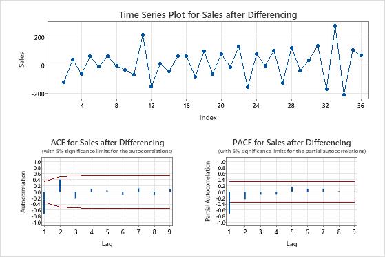
Plots of the differenced series
- Time series plot after differencing
- Use the time series plot of the differenced data to verify that differencing makes the mean of the data stationary. The time series plot shows the differences between consecutive observations. Data with a stationary mean follow a horizontal path on the time series plot.
- ACF plot and PACF plot after differencing
- Use the ACF of the differenced data to verify that differencing makes the mean of the data stationary. Plots with spikes that decrease quickly are characteristic of stationary data.
In these results, the time series plot shows that the mean and variance of the differenced data are approximately constant. The data appear to be stationary.
In the ACF plot of the differenced data, the only spike that is significantly different from 0 is at lag 1. This pattern also suggests that the data are stationary.