Forecast with Best ARIMA Model compares many models and selects a final model with a criterion in the specifications of the analysis. For information on the results for the final ARIMA model, go to Methods and formulas for ARIMA. The following sections contain details that are unique to Forecast with Best ARIMA Model.
Model selection
The model selection uses the following steps:
- Estimate the model parameters for every model. If a model includes a constant and the estimation of the parameters fails, try to estimate the parameters without the constant term.
- Calculate the information criterion for each model. The default criterion is the corrected Akaike Information Criterion (AICc).
- Produce results for the model with the best value of the information criterion.
The following sections describe details that differ in the selection of non-seasonal and seasonal models.
Non-seasonal models
- When you fit models with a constant term, candidate models have p + q ≤ 9.
- When you fit models without a constant term, candidate models have p + q ≤ 10.
- Models with d = 2 never include a constant term.
- The model evaluates ARIMA(0, d, 0) only when d = 1.
Seasonal models
- When you fit models with a constant term, candidate models have p + q + P + Q ≤ 9.
- When you fit models without a constant term, candidate models have p + q + P + Q ≤ 10.
- Models with d + D > 1 never include a constant term.
- The search for a seasonal model requires the order of at least one of the seasonal parameters to be able to be greater than 0. The search includes non-seasonal models if the specifications for the search include models where all the seasonal parameters have orders of 0.
- At least 1 of p, q, P, and Q is non-zero in every model.
Criteria
- Akaike Information Criterion (AIC)
- Corrected Akaike Information Criterion (AICc)
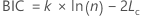
- Bayesian Information Criterion (BIC)
The calculation of the information criteria for a model uses the log-likelihood value for the model. The calculation of the log-likelihood value uses a recursive algorithm. For more information, see section 8.6 of Brockwell & Davis (1991)1.


Notation
| Term | Description |
|---|---|
| k | The number of
parameters in the model
|
| Lc | the log-likelihood of the current model |
| n | the sample size of the time series |
Box-Cox transformation
The analysis allows a Box-Cox transformation of the data. The transformation of the data happens before the model selection. For information on the Box-Cox transformation for time series data, go to Methods and formulas for Box-Cox Transformation for Time Series.
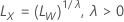
 for
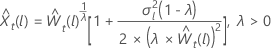
λ > 0
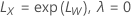
for
λ > 0
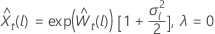
 for
λ = 0
for
λ = 0
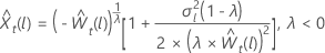
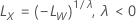
 for
λ < 0
for
λ < 0
where  is the tth value of the original time series and
t = 1, …,
n.
is the tth value of the original time series and
t = 1, …,
n.
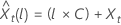
Let  be the
lth forecast value starting from the origin,
t, for the transformed data. Let
be the
lth forecast value starting from the origin,
t, for the transformed data. Let  be the
l-step forecast variance from the transformed data. Then, the
lth forecast value from
t for the original series depends on the value of
λ:
be the
l-step forecast variance from the transformed data. Then, the
lth forecast value from
t for the original series depends on the value of
λ:
where  is the limit in the original scale and
  is the limit in the transformed scale.
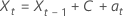
Random walk model
The ARIMA(0, 1, 0) model, with or without a constant term, is the random walk model. In Minitab Statistical Software, Forecast with Best ARIMA Model fits the random walk model. The command requires at least one autoregressive or moving average parameter. The estimation and probability limits for the random walk model have specific forms. The calculations for the loglikelihood, the forecast limits, and the probability limits for the forecasts depend on whether the model includes a constant term.
Definitions
| Term | Description |
|---|---|
 | the observations for a time series with t = 1, …, n |
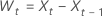
 | the first differenced data from the original time series,
 |

or

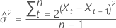
where  are independently and identically distributed and follow the normal
distribution with mean 0 and variance
σ2,
t = 2, …,
n.
are independently and identically distributed and follow the normal
distribution with mean 0 and variance
σ2,
t = 2, …,
n.
Equations that represent the model with a constant are similar:

or
Model without a constant term
The loglikelihood has the following form:
Loglikelihood
where

The 100 × (1 –
α) probability limit for the forecast value
 has the following form:
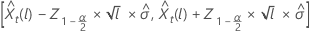
where  represents the 100 × (1 –
α/2)th percentile from the standard normal distribution.
represents the 100 × (1 –
α/2)th percentile from the standard normal distribution.
Model with a constant term
For a model with a constant, the calculations for the loglikelihood
require the estimation of the constant,
C. First, difference the data from the original series
 for
t = 2, …,
n. The constant is the sample mean of
for
t = 2, …,
n. The constant is the sample mean of
 and has the following form:

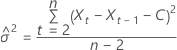
The loglikelihood has the following form:
Loglikelihood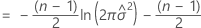
where
The 100 × (1 –
α) probability limit for the forecast value
 has the following form:

where  represents the 100 × (1 –
α/2)th percentile from the standard normal distribution.
represents the 100 × (1 –
α/2)th percentile from the standard normal distribution.