Step 1: Determine whether the data are stationary or trend stationary
The Augmented Dickey-Fuller Test table provides the hypotheses, a test statistic, a p-value, and a recommendation about whether to consider non-seasonal differencing to make the data stationary.
The test statistic provides one way to evaluate the null hypothesis. Test statistics that are less than or equal to the critical value provide evidence against the null hypothesis.
The p-value is a probability that measures the evidence against the null hypothesis. Lower probabilities provide stronger evidence against the null hypothesis.
To determine whether to difference the data, compare the test statistic to the critical value or the p-value to your significance level. Because the p-value contains more approximation, the recommendation from the analysis uses the critical value to assess the null hypothesis when the significance level is 0.01, 0.05, or 0.10. Usually, the conclusion is the same for the critical value and the p-value. The null hypothesis is that the data are non-stationary, which implies that differencing is a reasonable step to try to make the data stationary.
- P-value ≤ significance level
- Test statistic ≤ critical value
- If the p-value is less than or equal to the significance level or if the test statistic is less than or equal to the critical value, the decision is to reject the null hypothesis. Because the data provide evidence that the data are stationary, the recommendation of the analysis is to proceed without differencing.
- P-value > significance level
- Test statistic > critical value
- If the p-value is greater than the significance level or if the test statistic is greater than the critical value, the decision is to fail to reject the null hypothesis. Because the data do not provide evidence that the data are stationary, the recommendation of the analyis is to determine whether differencing makes the mean of the data stationary.
If the data are stationary, the test does not recommend differencing. Explore ARIMA models that do not include any differencing terms. If the data are not stationary, then explore ARIMA models that include differencing terms. Use the time series plot of the differenced data to see whether the differences between consecutive observations are a stationary set of data. If the differenced data are stationary, then ARIMA models with a first order term for differencing are reasonable to consider.
In these results, the test statistic of 2.29045 is greater than the critical value of approximately -2.96053. Because the results fail to reject the null hypothesis that the data are non-stationary, the recommendation of the test is to consider differencing to make the data stationary.
Augmented Dickey-Fuller Test
| Null hypothesis: | Data are non-stationary |
|---|---|
| Alternative hypothesis: | Data are stationary |
| Test Statistic | P-Value | Recommendation |
|---|---|---|
| 2.29045 | 0.999 | Test statistic > critical value of -2.96053. |
| Significance level = 0.05 | ||
| Fail to reject null hypothesis. | ||
| Consider differencing to make data stationary. |
Step 2: Examine the effect of differencing the data
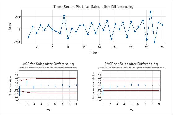
When the conclusion of the test supports differencing, examine the plots of the differenced data for characteristics of data that are not stationary. A trend in the time series plot is an example of a pattern that indicates that the mean of the data is not stationary. On the ACF plot, large spikes that decrease slowly also indicate data that are not stationary. If you see these patterns in the differenced data, then consider whether to fit an ARIMA model with a second order of differencing. Usually, 1 or 2 orders of differencing are enough to provide a reasonable fit to the data.
If the differenced data are stationary, then a reasonable approach is to include a single order of non-seasonal differencing in an ARIMA model. For more information on ARIMA models, go to Overview for ARIMA.
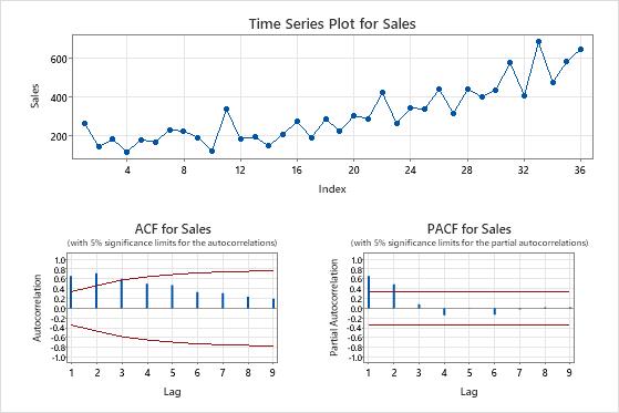
The time series plots show the result of the differencing. In these results, the time series plot of the original data shows a clear trend. The time series plot of the differenced data shows the differences between consecutive values. The differenced data appear stationary because the points follow a horizontal path without obvious patterns in the variation.
The ACF plots also show the effect of differencing. In these results, the ACF plot of the original data shows slowly-decreased spikes across lags. This pattern indicates that the data are not stationary. In the ACF plot of the differenced data, the only spike that is significantly different from 0 is at lag 1.
In these results, the time series plots and the ACF plots confirm the test results. Therefore, a reasonable approach is to difference the data and then fit an autoregressive and moving average model to make forecasts.