A marketing analyst wants to use an ARIMA model to generate short-term forecasts for sales of a shampoo product. The analyst collects sales data from the previous three years. On a time series plot, the analyst sees that the data trend higher. This pattern indicates that the mean of the data is not stationary. The analyst performs an augmented Dickey-Fuller test to determine the order of non-seasonal differencing to include in the ARIMA model. For more information on ARIMA models, go to Overview for ARIMA.
- Open the sample data ShampooSales.MWX.
- Choose .
- In Series, enter Sales.
- Select OK.
Interpret the results
In these results, the test statistic of 2.29045 is greater than the critical value of -2.96053. Because the results fail to reject the null hypothesis that the data are non-stationary, the recommendation of the test is to consider first-order differencing to make the data stationary.
Method
| Maximum lag order for terms in the regression model | 9 |
|---|---|
| Criterion for selecting lag order | Minimum AIC |
| Additional terms | Constant |
| Selected lag order | 4 |
| Rows used | 36 |
Augmented Dickey-Fuller Test
| Null hypothesis: | Data are non-stationary |
|---|---|
| Alternative hypothesis: | Data are stationary |
| Test Statistic | P-Value | Recommendation |
|---|---|---|
| 2.29045 | 0.999 | Test statistic > critical value of -2.96053. |
| Significance level = 0.05 | ||
| Fail to reject null hypothesis. | ||
| Consider differencing to make data stationary. |
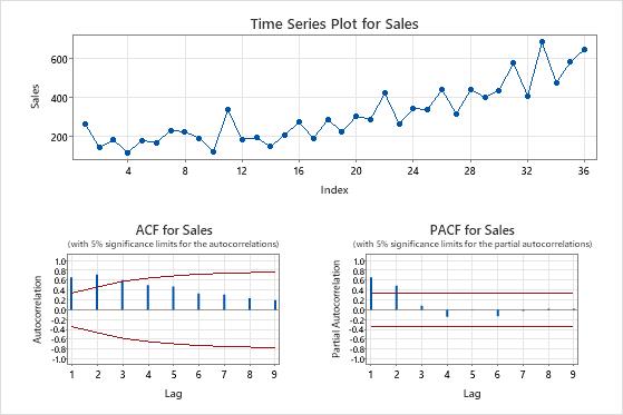
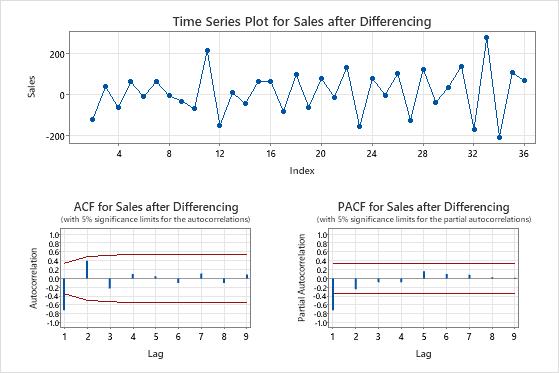
The time series plots show the result of the differencing. In these results, the time series plot of the original data shows a clear trend. The time series plot of the differenced data shows the differences between consecutive values. The differenced data appear stationary because the points follow a horizontal path without obvious patterns in the variation.
The ACF plots also show the effect of differencing. In these results, the ACF plot of the original data shows slowly-decreased spikes across lags. This pattern indicates that the data are not stationary. In the ACF plot of the differenced data, the only spike that is significantly different from 0 is at lag 1.
In these results, the time series plots and the ACF plots confirm the test results. Therefore, a reasonable approach is to difference the data and then fit an autoregressive and moving average model to make forecasts.