In This Topic
Fully Nested ANOVA model
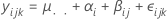
The nested ANOVA model for a balanced design with two random factors (A and B) is:
yijk = μ .. + α i+ β j(i) +εijk
where α i, β j(i) , and ε ijkare independent normal random variables with expectations 0 and variances σ2 α, σ2 β, and σ2, respectively.
The parameters are estimated by the following:
μ .. = y̅...
α i = yi..− y̅...
β j(i) = yij.− y̅i..
where y̅... = mean of all observations, yi.. = mean of observations at the ith level of factor A, yij. = is the mean of observations for the jth level of factor B at the ith level of factor A. The parameter β j(i) is the specific effect of B when A is at the ith level.
- J. Neter, W. Wasserman and M.H. Kutner (1985). Applied Linear Statistical Models. Second Edition. Irwin, Inc.
Sequential sum of squares
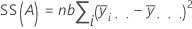
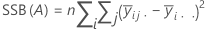
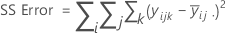
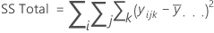
The sum of squared distances. SS Total is the total variation in the data. SS (A) and SS (B) is the amount of variation of the estimated factor level mean around the overall mean. They are also known as the sum of squares for factor A or factor B. SS Error is the amount of variation of the observations from their fitted values. The calculations are:

Minitab provides the sequential sum of squares, which depend on the order in which the factors are entered into the model. It is the unique portion of SS Regression explained by a factor, given any previously entered factors.
Notation
| Term | Description |
|---|---|
| a | number of levels in factor A |
| b | number of levels in factor B |
| n | total number of trials |
| yi.. | mean of the ith factor level of factor A |
| y... | overall mean of all observations |
| y.j. | mean of the jth factor level of factor B |
| yij. | mean of observations at the ith level of factor A and the jth level of factor B |
Degrees of freedom (DF)
For a fully nested ANOVA model with two factors, A and B, the degrees of freedom are:

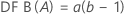
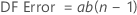
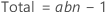
where a = the number of levels in factor A, b = the number of levels in factor B, and n is the number of trials.
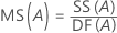
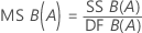
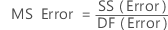
Mean square (MS)
Formulas
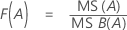
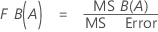
F
These are the formulas for F statistics for a model with random factors.
Formulas
P-value – Analysis of variance table
The p-value is a probability that is calculated from an F-distribution with the degrees of freedom (DF) as follows:
- Numerator DF
- sum of the degrees of freedom for the term or the terms in the test
- Denominator DF
- degrees of freedom for error
Formula
1 − P(F ≤ fj)
Notation
| Term | Description |
|---|---|
| P(F ≤ f) | cumulative distribution function for the F-distribution |
| f | f-statistic for the test |
Variance components
Calculated for random factors. The nested model with two random factor is:
where, αi, βj(i), and εijk are independent normal random variables. The variables are normally distributed with mean zero and variances given by V(αi) = σ2α,V(βj) = σ2β, and V(εijk) = σ2. It is assumed that all bj(i) have the same variance σ2β, σ2α, σ2β, σ2αβ, σ2 are called variance components.
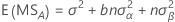
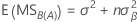
Expected mean squares
For a model with two random factors, A and B, the expected mean squares are:

F-statistic for models with random factors
How the F-statistics in the ANOVA output are calculated
Each F-statistic is a ratio of mean squares. The numerator is the mean square for the term. The denominator is chosen such that the expected value of the numerator mean square differs from the expected value of the denominator mean square only by the effect of interest. The effect for a random term is represented by the variance component of the term. The effect for a fixed term is represented by the sum of squares of the model components associated with that term divided by its degrees of freedom. Therefore, a high F-statistic indicates a significant effect.
When all the terms in the model are fixed, the denominator for each F-statistic is the mean square of the error (MSE). However, for models that include random terms, the MSE is not always the correct mean square. The expected mean squares (EMS) can be used to determine which is appropriate for the denominator.
Example
| Source | Expected Mean Square for Each Term |
|---|---|
| (1) Screen | (4) + 2.0000(3) + Q[1] |
| (2) Tech | (4) + 2.0000(3) + 4.0000(2) |
| (3) Screen*Tech | (4) + 2.0000(3) |
| (4) Error | (4) |
A number with parentheses indicates a random effect associated with the term listed beside the source number. (2) represents the random effect of Tech, (3) represents the random effect of the Screen*Tech interaction, and (4) represents the random effect of Error. The EMS for Error is the effect of the error term. In addition, the EMS for Screen*Tech is the effect of the error term plus two times the effect of the Screen*Tech interaction.
To calculate the F-statistic for Screen*Tech, the mean square for Screen*Tech is divided by the mean square of the error so that the expected value of the numerator (EMS for Screen*Tech = (4) + 2.0000(3)) differs from the expected value of the denominator (EMS for Error = (4)) only by the effect of the interaction (2.0000(3)). Therefore, a high F-statistic indicates a significant Screen*Tech interaction.
A number with Q[ ] indicates the fixed effect associated with the term listed beside the source number. For example, Q[1] is the fixed effect of Screen. The EMS for Screen is the effect of the error term plus two times the effect of the Screen*Tech interaction plus a constant times the effect of Screen. Q[1] equals (b*n * sum((coefficients for levels of Screen)**2)) divided by (a - 1), where a and b are the number of levels of Screen and Tech, respectively, and n is the number of replicates.
To calculate the F-statistic for Screen, the mean square for Screen is divided by the mean square for Screen*Tech so that the expected value of the numerator (EMS for Screen = (4) + 2.0000(3) + Q[1] ) differs from the expected value of the denominator (EMS for Screen*Tech = (4) + 2.0000(3) ) only by the effect due to the Screen (Q[1]). Therefore, a high F-statistic indicates a significant Screen effect.
Why does my ANOVA output include an "x" beside a p-value in the ANOVA table and the label "Not an exact F-test"?
An exact F-test for a term is one in which the expected value of the numerator mean squares differs from the expected value of the denominator mean squares only by the variance component or the fixed factor of interest.
Sometimes, however, such a mean square cannot be calculated. In this case, Minitab uses a mean square that results in an approximate F-test and displays an "x" beside the p-value to identify that the F-test is not exact.
| Source | Expected Mean Square for Each Term |
|---|---|
| (1) Supplement | (4) + 1.7500(3) + Q[1] |
| (2) Lake | (4) + 1.7143(3) + 5.1429(2) |
| (3) Supplement*Lake | (4) + 1.7500(3) |
| (4) Error | (4) |
The F-statistic for Supplement is the mean square for Supplement divided by the mean square for the Supplement*Lake interaction. If the effect for Supplement is very small, the expected value of the numerator equals the expected value of the denominator. This is an example of an exact F-test.
Notice, however, that for a very small Lake effect, there are no mean squares such that the expected value of the numerator equals the expected value of the denominator. Therefore, Minitab uses an approximate F-test. In this example, the mean square for Lake is divided by the mean square for the Supplement*Lake interaction. This results in an expected value of the numerator being approximately equal to that of the denominator if the Lake effect is very small.
About the "Denominator of F-test is zero or undefined" message
- There is not at least one degree of freedom for error.
-
The adjusted MS values are very small, and thus there is not enough precision to display the F and p-values. As a workaround, multiply the response column by 10. Then perform the same regression model, but instead use this new response column for the response.
Note
Multiplying the response values by 10 will not affect the F and p-values that Minitab displays the output. However, decimal position will be affected in the remaining output, specifically, the sequential sums of squares, Adj SS, Adj MS, Fit, standard error of the fits, and residual columns.