In This Topic
Sample statistics
Formula

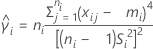
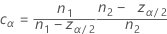
Notation
| Term | Description |
|---|---|
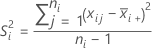
 | mean of sample i |
| S2i | variance of sample i |
| Xij | jth measurement of the ith sample |
| ni | size of sample i |
Test for Bonett's method with balanced designs
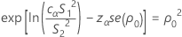
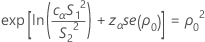
Formula for the test statistic
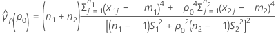
When n1 = n2 , the test statistic is Z2. If the null hypothesis, ρ = ρ0 is true, then Z2 is distributed as a chi-square distribution with 1 degree of freedom. Z2 is given by:
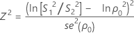
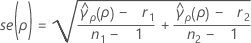
where se(ρ0) is the standard error of the pooled kurtosis, which is given by:
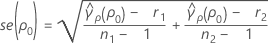
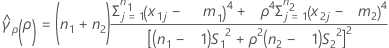
where ri = ( ni - 3) / ni and  is the pooled kurtosis, which is given by:

se2(ρ0) can also be expressed in terms of the kurtosis values of the individual samples,  , as follows:
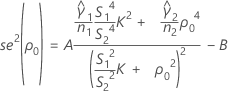
where:

Formula for p-value
Let z2 be the value of Z2 that is obtained from the data. Under the null hypothesis, H0: ρ = ρ0 , Z is distributed as the standard normal distribution. Therefore, the p-values for the alternative hypotheses (H1) are given by the following.
| Hypothesis | P-value |
|---|---|
| H1: ρ0 ≠ ρ0 | P = 2P(Z > |z|) |
| H1: ρ0 > ρ0 | P = P(Z > z) |
| H1: ρ0 < ρ0 | P = P(Z < z) |
Notation
| Term | Description |
|---|---|
| Si | the standard deviation of sample i |
| ρ | the ratio of the population standard deviations |
| ρ0 | the hypothesized ratio of the population standard deviations |
| α | the significance level for the test = 1 - (the confidence level / 100) |
| ni | the number of observations in sample i |
 | the kurtosis value for sample i |
| Xij | the jth observation in sample i |
| mi | the trimmed mean for sample i with trim proportions of  |
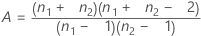
Test for Bonett's method with unbalanced designs
Formula
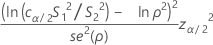
When n1 ≠ n2 , there is no test statistic. Rather, the p-value is calculated by inverting the confidence interval procedure. The p-value for the test is given by:
P = 2 min (αL, αU)
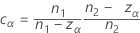
where cα is an equalizer constant described below and se(ρ0) is the standard error of the pooled kurtosis, which is given by:

where ri = (ni - 3) / ni and  is the pooled kurtosis which is given by:
se(ρ0) can also be expressed in terms of the kurtosis values of the individual samples. For more information go to Test for Bonett's method with balanced designs.
Equalizer constant
The constant vanishes when the designs are balanced, and its effect becomes negligible with increasing sample sizes.
Finding αL and αU
Finding αL and αU is equivalent to finding the roots of the functions L(z , n1 , n2 , S1 , S2 ) and L(z , n2 , n1 , S2 , S1 ), where L(z , n1 , n2 , S1 , S2) is given by:

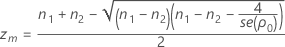
- Calculate zm and evaluate L(z, n1, n2, S1, S2).
- If L(zm)
 0, then find the root zL, of L(z, n1, n2, S1, S2) in the interval
  and calculate αL = P( Z > zL).
 - If L(zm) > 0, then the function L(z , n1, n2, S1, S2) has no root, and αL = 0.
- If L(zm)
- Calculate L(0, n1, n2, S1, S2) = ln (S12 / S22).
- If L(0, n1, n2, S1, S2)
 0, then find the root z0, of L(z, n1, n2, S1, S2) in the interval [0, n2).
 - If L(0, n1, n2, S1, S2) < 0, then find the root zL in the interval
 .
.
- If L(0, n1, n2, S1, S2)
- Calculate αL = P( Z > zL).
To calculate αU, apply the previous steps using the function, L(z, n2, n1, S2, S1), instead of the function, L(z, n1, n2, S1, S2).
Notation
| Term | Description |
|---|---|
| Si | the standard deviation of sample i |
| ρ | the ratio of the population standard deviations |
| ρ0 | the hypothesized ratio of the population standard deviations |
| α | the significance level for the test = 1 - (the confidence level / 100) |
| zα | the upper α percentile point of the standard normal distribution |
| ni | the number of observations in sample i |
| Xij | the jth observation in sample i |
| mi | the trimmed mean for sample i with trim proportions of  |
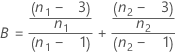
Confidence interval for Bonett's method
Formula
where cα/2 is an equalizer constant (described below) and se(ρ) is the standard error of the pooled kurtosis (described below). Typically, this equation has two solutions, a solution, L < S1 / S2, and a solution U > S1 / S2. L is the lower confidence limit, and U is the upper confidence limit. For more information, go to Bonett's Method, which is a white paper that has simulations and other information about Bonett's Method.
The confidence limits for the ratio of the variances are obtained by squaring the confidence limits for the ratio of the standard deviations.
Equalizer constant
The constant vanishes when the designs are balanced, and its effect becomes negligible with increasing sample sizes.
Standard error of the pooled kurtosis
se(ρ) is the standard error of the pooled kurtosis which is given by:
where ri = (ni - 3) / ni and  is the pooled kurtosis which is given by:
se(ρ) can also be expressed in terms of the kurtosis values of the individual samples. For more information, see the section on the Test for Bonett's method with balanced designs.
Notation
| Term | Description |
|---|---|
| α | the significance level for the test = 1 - (the confidence level / 100) |
| Si | the standard deviation of sample i |
| ρ | the ratio of the population standard deviations |
| zα/2 | the upper α/2 percentile point of the standard normal distribution |
| ni | the number of observations in sample i |
| Xij | the jth observation in sample i |
| mi | the trimmed mean for sample i with trim proportions of  |
Test for Levene's method
Formula
Levene’s test is appropriate for continuous data. Levene’s test is not available for summarized data.
To test the null hypothesis that σ1 / σ2 = ρ with Levene’s test, Minitab performs a one-way ANOVA on the values Z1j and ρZ2j (where j = 1, …, n1 or n2).
The Levene's test statistic equals the value of the F-statistic in the resulting ANOVA table. The Levene's test p-value equals the p-value in this ANOVA table.
- H. Levene (1960). Contributions to Probability and Statistics. Stanford University Press, CA.
- M.B. Brown and A.B. Forsythe (1974). "Robust Tests for the Equality of Variance," Journal of the American Statistical Association, 69, 364–367.
Degrees of freedom
Under the null hypothesis, the test statistic follows an F-distribution with degrees of freedom DF1 and DF2.
DF1 = 1
DF2 = n1 + n2 – 2
Notation
| Term | Description | ||||||||||
|---|---|---|---|---|---|---|---|---|---|---|---|
| Zij | |Xi j – η i|
| ||||||||||
| σ1 | standard deviation of the first population | ||||||||||
| σ2 | standard deviation of the second population | ||||||||||
| n1 | size of the first sample | ||||||||||
| n2 | size of the second sample |
Confidence intervals for Levene's method
Formula
For continuous data, Minitab calculates the confidence limits for the ratio (ρ) between the population standard deviations with the following formulas. To obtain limits for the ratio between population variances, square the values below.
-
If
 , lower limit =
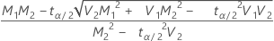
If
 , a lower limit does not exist
 -
If
 , upper limit =
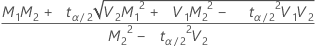
If
 , an upper limit does not exist
-
If
 , then
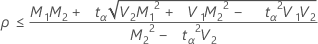
- If
 , an upper bound does not exist
-
If
 , then
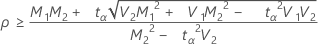
- If
 , a lower bound does not exist
Notation
| Term | Description |
|---|---|
| t α | the α critical value of a t distribution with n1 + n2 – 2 degrees of freedom |
| ηi | the median of sample i |
| Zij |  where j = 1, 2, ... , ni and i = 1, 2, and Xij are individual observations where j = 1, 2, ... , ni and i = 1, 2, and Xij are individual observations |
| Mi | the mean of Zij |
| Si2 | the sample variance of Zij |
| vi | 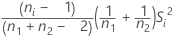 |
| ρ | σ1 / σ2 |
| n1 | the size of the first sample |
| n2 | the size of the second sample |
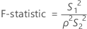
Test for the F-test method
The F-test is appropriate for normal data. To test the null hypothesis that σ1 / σ2 = ρ with the F-test, Minitab uses the following formulas.
Formula for the test statistic
Formula for degrees of freedom
Under the null hypothesis, the F-statistic follows an F-distribution with degrees of freedom DF1 and DF2.
DF1 = n1 – 1
DF2 = n2 – 1
Formula for p-value
- For a one-sided test with an alternative hypothesis of less than, the p-value equals the probability of obtaining an F-statistic that is equal to or less than the observed value from an F-distribution with degrees of freedom DF1 and DF2.
- For a two-sided test where the ratio is less than 1, the p-value equals two times the area under the F-curve less than the observed value from an F-distribution with degrees of freedom DF1 and DF2.
- For a two-sided test where the ratio is greater than 1, the p-value equals two times the area under the F-curve greater than the observed value from an F-distribution with degrees of freedom DF1 and DF2.
- For a one-sided test with an alternative hypothesis of greater than, the p-value equals the probability of obtaining an F-statistic that is equal to or greater than the observed value from an F-distribution with degrees of freedom DF1 and DF2.
Notation
| Term | Description |
|---|---|
| ρ | σ1 / σ2 |
| σ1 | standard deviation of the first population |
| σ2 | standard deviation of the second population |
| S21 | variance of the first sample |
| S22 | variance of the second sample |
| n1 | size of the first sample |
| n2 | size of the second sample |
Confidence intervals for the F-test method
When the data follow a normal distribution, Minitab calculates the confidence bounds for the ratio (ρ) between the population standard deviations with the following formulas. To obtain bounds for the ratio between population variances, square the values below.
Formula
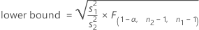
When you specify a "not equal" alternative hypothesis, a 100(1 – α)% confidence interval for ρ is given by:
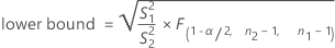

When you specify a "less than" alternative hypothesis, a 100(1 – α)% upper confidence bound for ρ is given by:
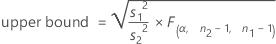
When you specify a "greater than" alternative hypothesis, a 100(1 – α)% lower confidence bound for ρ is given by:
Notation
| Term | Description |
|---|---|
| S1 | standard deviation of the first sample |
| S2 | standard deviation of the second sample |
| ρ | σ1 / σ2 |
| n1 | size of the first sample |
| n2 | size of the second sample |
| F(α/2, n2–1, n1–1) | α/2 critical value from the F-distribution with degrees of freedom n2–1 and n1–1. |