In This Topic
Power for difference
The first line of output indicates how the hypotheses are specified for the equivalence test.
"Power for difference" indicates that the hypotheses are specified in terms of the difference between the mean of the test population and the target value (Test mean – target).
Null hypothesis and alternative hypothesis
- Null hypothesis
- Minitab tests one or both of the following null hypotheses, depending on the alternative hypothesis that you selected:
- The difference between the population mean and the target is greater than or equal to the upper equivalence limit.
- The difference between the population mean and the target is less than or equal to the lower equivalence limit.
- Alternative hypothesis
- The alternative hypothesis states either or both of the following:
- The difference between the population mean and the target is less than the upper equivalence limit.
- The difference between the population mean and the target is greater than the lower equivalence limit.
Interpretation
Use the null and alternative hypotheses to verify that the equivalence criteria are correct and that you have selected the appropriate alternative hypothesis to test.
Method
| Power for difference: | Test mean - target |
|---|---|
| Null hypothesis: | Difference ≤ -0.42 or Difference ≥ 0.42 |
| Alternative hypothesis: | -0.42 < Difference < 0.42 |
| α level: | 0.05 |
| Assumed standard deviation: | 0.332 |
- The difference between the population mean and the target is less than or equal to the lower equivalence limit of −0.42
- The difference between the population mean and the target is greater than or equal to the upper equivalence limit of 0.42
α (alpha)
The significance level (denoted by alpha or α) is the maximum acceptable level of risk for rejecting the null hypothesis when the null hypothesis is true (type I error). For example, if you perform an equivalence test using the default hypotheses, an α of 0.05 indicates a 5% risk of claiming equivalence when the difference between the mean and the target does not actually fall within the equivalence limits.
The α-level for an equivalence test also determines the confidence level for the confidence interval. The confidence level is 1 – α by default, or 1 – 2α if you use the alternative method of calculating the confidence interval.
Interpretation
Use the significance level to minimize the power value of the test when the null hypothesis (H0) is true. Higher values for the significance level give the test more power, but also increase the chance of making a type I error, which is rejecting the null hypothesis when it is true.
Assumed standard deviation
The standard deviation is the most common measure of dispersion, or how much the data vary relative to the mean. Variation that is random or natural to a process is often referred to as noise.
Interpretation
The assumed standard deviation is a planning estimate of the population standard deviation that you enter for the power analysis. Minitab uses the assumed standard deviation to calculate the power of the test. Higher values of the standard deviation indicate that there is more variation in the data, which decreases the statistical power of a test.Difference
This value represents the difference between the population mean and the target.
Note
The definitions and interpretation in this topic apply to a standard equivalence test that uses the default alternative hypothesis (Lower limit < test mean - target < upper limit).
Interpretation
If you enter the sample size and the power of the test, then Minitab calculates the difference that the test can accommodate at the specified power and sample size. For larger sample sizes, the difference can be closer to your equivalence limits.
To more fully investigate the relationship between the sample size and the difference that the test can accommodate at a given power, use the power curve.
Method
| Power for difference: | Test mean - target |
|---|---|
| Null hypothesis: | Difference ≤ -0.42 or Difference ≥ 0.42 |
| Alternative hypothesis: | -0.42 < Difference < 0.42 |
| α level: | 0.05 |
| Assumed standard deviation: | 0.732 |
Results
| Sample Size | Power | Difference |
|---|---|---|
| 30 | 0.9 | * |
| 40 | 0.9 | -0.071272 |
| 40 | 0.9 | 0.071272 |
| 60 | 0.9 | -0.140212 |
| 60 | 0.9 | 0.140212 |
| 100 | 0.9 | -0.204306 |
| 100 | 0.9 | 0.204306 |
These results show how increasing the sample size increases the size of the difference that can be accommodated at a given power level:
- With 30 observations, you cannot achieve a power of 0.9 to claim equivalence, regardless of the difference.
- With 40 observations, the power of the test is at least 0.9 when the difference is between approximately −0.07 and 0.07.
- With 60 observations, the power of the test is at least 0.9 when the difference is between approximately −0.14 and 0.14.
- With 100 observations, the power of the test is at least 0.9 when the difference is between approximately −0.20 and 0.20.
Sample Size
The sample size is the total number of observations in the sample.
Interpretation
Use the sample size to estimate how many observations you need to obtain a certain power value for the equivalence test at a specific difference.
If you enter a difference and a power value for the test, then Minitab calculates how large your sample must be.Because sample sizes are whole numbers, the actual power of the test might be slightly greater than the power value that you specify.
If you increase the sample size, the power of the test also increases. You want enough observations in your sample to achieve adequate power. But you don't want a sample size so large that you waste time and money on unnecessary sampling or detect unimportant differences to be statistically significant.
To more fully investigate the relationship between the sample size and the difference that the test can accommodate at a given power, use the power curve.
Method
| Power for difference: | Test mean - target |
|---|---|
| Null hypothesis: | Difference ≤ -0.42 or Difference ≥ 0.42 |
| Alternative hypothesis: | -0.42 < Difference < 0.42 |
| α level: | 0.05 |
| Assumed standard deviation: | 0.732 |
Results
| Difference | Sample Size | Target Power | Actual Power |
|---|---|---|---|
| 0.1 | 47 | 0.9 | 0.903687 |
| 0.2 | 97 | 0.9 | 0.902206 |
| 0.3 | 321 | 0.9 | 0.900788 |
These results show that, as the size of the difference increases and approaches the value of the equivalence limit, you need a larger sample size to achieve a given power. If the difference is 0.1, then you need at least 47 observations to achieve a power of 0.9. If the difference is 0.3, you need at least 321 observations to achieve a power of 0.9.
Power
Note
The definitions and interpretation in this topic apply to a standard equivalence test that uses the default alternative hypothesis (Lower limit < test mean - target < upper limit).
The power of an equivalence test is the probability that the test will demonstrate that the difference is within your equivalence limits, when it actually is. The power of an equivalence test is affected by the sample size, the difference, the equivalence limits, the variability of the data, and the significance level of the test.
For more information, go to Power for equivalence tests.
Interpretation
If you enter a sample size and a difference, then Minitab calculates the power of the test. A power value of 0.9 is usually considered adequate. A power of 0.9 indicates that you have a 90% chance of demonstrating equivalence when the population difference is actually within the equivalence limits. If an equivalence test has low power, you might fail to demonstrate equivalence even when the population mean and the target are equivalent.
If you enter a difference and a power value for the test, then Minitab calculates how large your sample must be. Minitab also calculates the actual power of the test for that sample size. Because sample sizes are whole numbers, the actual power of the test might be slightly greater than the power value that you specify.
Usually, when the sample size is smaller or the difference is closer to an equivalence limit, the test has less power to claim equivalence.
Method
| Power for difference: | Test mean - target |
|---|---|
| Null hypothesis: | Difference ≤ -0.42 or Difference ≥ 0.42 |
| Alternative hypothesis: | -0.42 < Difference < 0.42 |
| α level: | 0.05 |
| Assumed standard deviation: | 0.732 |
Results
| Difference | Sample Size | Power |
|---|---|---|
| 0.1 | 20 | 0.516387 |
| 0.1 | 35 | 0.806390 |
| 0.2 | 20 | 0.341093 |
| 0.2 | 35 | 0.538352 |
In these results, for a difference of 0.1, the power of the test is approximately 0.52 with a sample size of 20, and 0.81 with a sample size of 35. For a difference of 0.2, the power is approximately 0.34 with a sample size of 20, and 0.54 with a sample size of 35.
Power curve
The power curve plots the power of the test versus the difference between the mean and the target.
Interpretation
Use the power curve to assess the appropriate sample size or power for your test.
The power curve represents every combination of power and difference for each sample size when the significance level and the standard deviation are held constant. Each symbol on the power curve represents a calculated value based on the values that you enter. For example, if you enter a sample size and a power value, Minitab calculates the corresponding difference and displays the calculated value on the graph.
Examine the values on the curve to determine the difference between the mean and the target that can be accommodated at a certain power value and sample size. A power value of 0.9 is usually considered adequate. However, some practitioners consider a power value of 0.8 to be adequate. If an equivalence test has low power, you might fail to demonstrate equivalence even when the mean is equivalent to the target. If you increase the sample size, the power of the test also increases. You want enough observations in your sample to achieve adequate power. But you don't want a sample size so large that you waste time and money on unnecessary sampling or detect unimportant differences to be statistically significant. Usually, differences that are closer to the equivalence limits require more power to demonstrate equivalence.
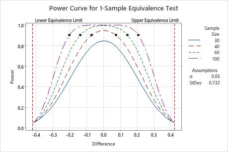
In this graph, the power curve for a sample size of 30 shows that the test cannot achieve a power of 0.9 for any size difference. The power curve for a sample size of 40 shows the test has power of 0.9 for a difference of approximately 0.0. The power curve for a sample size of 100 shows that the test has a power of 0.9 for a difference of approximately ±0.2. For each curve, as the difference approaches the lower equivalence limit or upper equivalence limit, the power of the test decreases and approaches α (alpha, which is the risk of claiming equivalence when it is not true).