A quality engineer for a building products manufacturer is developing a new insulation product. The engineer designs a 2-level full factorial experiment to study the effects of several factors on the variability in insulation strength. While conducting the strength experiment, the engineer decides to collect extra samples to examine the effects of the factors on the variability in insulation strength. The engineer collects six repeat measurements of strength at each combination of factor settings and calculates the standard deviation of the repeats.
The engineer analyzes the variability in a factorial design to determine how material type, injection pressure, injection temperature, and cooling temperature affect the variability in the strength of the insulation.
- Open the sample data, InsulationStrength.MWX.
- Complete Example of Pre-Process Responses for Analyze Variability.
- Choose .
- In Response (standard deviations), enter Std.
- Click Terms.
- In Include terms in the model up through order, choose 2 from the drop-down list. Click OK.
- Click Graphs.
- Under Effects Plots, select Pareto.
- Under Residual Plots, select Three in one.
- Click OK in each dialog box.
Interpret the results
In the Analysis of Variance table, the p-value for the main effect for Material and the interaction Material*InjPress are significant at the α-level of 0.05. The engineer can consider reducing the model.
The R2 value shows that the model explains 97.75% of the variance in strength, which indicates that the model fits the data extremely well.
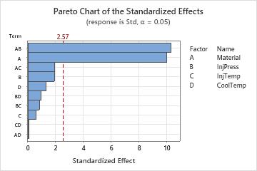
The Pareto plot of the effects allows you to visually identify the important effects and compare the relative magnitude of the various effects. In addition, you can see that the largest effect is Material*InjPress (AB) because it extends the farthest. Material*CoolTemp (AD) is the smallest because it extends the least.
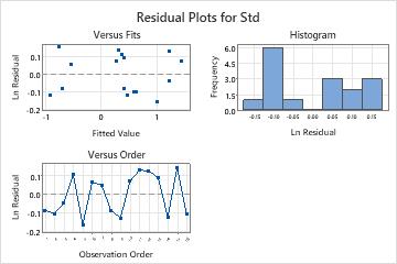
The residual plots do not indicate any problems with the model.
Method
| Estimation | Least squares |
|---|
Coded Coefficients for Ln(Std)
| Term | Effect | Ratio Effect | Coef | SE Coef | T-Value | P-Value | VIF |
|---|---|---|---|---|---|---|---|
| Constant | 0.3424 | 0.0481 | 7.12 | 0.001 | |||
| Material | -0.9598 | 0.3830 | -0.4799 | 0.0481 | -9.99 | 0.000 | 1.00 |
| InjPress | -0.1845 | 0.8315 | -0.0922 | 0.0481 | -1.92 | 0.113 | 1.00 |
| InjTemp | 0.0555 | 1.0571 | 0.0278 | 0.0481 | 0.58 | 0.589 | 1.00 |
| CoolTemp | -0.1259 | 0.8817 | -0.0629 | 0.0481 | -1.31 | 0.247 | 1.00 |
| Material*InjPress | -0.9918 | 0.3709 | -0.4959 | 0.0481 | -10.32 | 0.000 | 1.00 |
| Material*InjTemp | 0.1875 | 1.2062 | 0.0937 | 0.0481 | 1.95 | 0.109 | 1.00 |
| Material*CoolTemp | 0.0056 | 1.0056 | 0.0028 | 0.0481 | 0.06 | 0.956 | 1.00 |
| InjPress*InjTemp | -0.0792 | 0.9239 | -0.0396 | 0.0481 | -0.82 | 0.448 | 1.00 |
| InjPress*CoolTemp | -0.0900 | 0.9139 | -0.0450 | 0.0481 | -0.94 | 0.392 | 1.00 |
| InjTemp*CoolTemp | 0.0066 | 1.0066 | 0.0033 | 0.0481 | 0.07 | 0.948 | 1.00 |
Model Summary for Ln(Std)
| S | R-sq | R-sq(adj) | R-sq(pred) |
|---|---|---|---|
| 0.549040 | 97.75% | 93.25% | 76.97% |
Analysis of Variance for Ln(Std)
| Source | DF | Adj SS | Adj MS | F-Value | P-Value |
|---|---|---|---|---|---|
| Model | 10 | 65.4970 | 6.5497 | 21.73 | 0.002 |
| Linear | 4 | 31.7838 | 7.9459 | 26.36 | 0.001 |
| Material | 1 | 30.0559 | 30.0559 | 99.71 | 0.000 |
| InjPress | 1 | 1.1104 | 1.1104 | 3.68 | 0.113 |
| InjTemp | 1 | 0.1005 | 0.1005 | 0.33 | 0.589 |
| CoolTemp | 1 | 0.5170 | 0.5170 | 1.71 | 0.247 |
| 2-Way Interactions | 6 | 33.7132 | 5.6189 | 18.64 | 0.003 |
| Material*InjPress | 1 | 32.0953 | 32.0953 | 106.47 | 0.000 |
| Material*InjTemp | 1 | 1.1466 | 1.1466 | 3.80 | 0.109 |
| Material*CoolTemp | 1 | 0.0010 | 0.0010 | 0.00 | 0.956 |
| InjPress*InjTemp | 1 | 0.2046 | 0.2046 | 0.68 | 0.448 |
| InjPress*CoolTemp | 1 | 0.2642 | 0.2642 | 0.88 | 0.392 |
| InjTemp*CoolTemp | 1 | 0.0014 | 0.0014 | 0.00 | 0.948 |
| Error | 5 | 1.5072 | 0.3014 | ||
| Total | 15 | 67.0043 |
Regression Equation in Uncoded Units
| Ln(Std) | = | -1.30 - 0.158 Material + 0.0148 InjPress + 0.0180 InjTemp + 0.0031 CoolTemp - 0.01322 Material*InjPress + 0.01250 Material*InjTemp + 0.00028 Material*CoolTemp - 0.000141 InjPress*InjTemp - 0.000120 InjPress*CoolTemp + 0.000044 InjTemp*CoolTemp |
|---|
Alias Structure
| Factor | Name |
|---|---|
| A | Material |
| B | InjPress |
| C | InjTemp |
| D | CoolTemp |
| Aliases |
|---|
| I |
| A |
| B |
| C |
| D |
| AB |
| AC |
| AD |
| BC |
| BD |
| CD |