When you want to determine information about a particular population characteristic (for example, the mean), you usually take a random sample from that population because it is infeasible to measure the entire population. Using that sample, you calculate the corresponding sample characteristic, which is used to summarize information about the unknown population characteristic. The population characteristic of interest is called a parameter and the corresponding sample characteristic is the sample statistic or parameter estimate. Because the statistic is a summary of information about a parameter obtained from the sample, the value of a statistic depends on the particular sample that was drawn from the population. Its values change randomly from one random sample to the next one, therefore a statistic is a random quantity (variable). The probability distribution of this random variable is called sampling distribution. The sampling distribution of a (sample) statistic is important because it enables us to draw conclusions about the corresponding population parameter based on a random sample.
For example, when we draw a random sample from a normally distributed population, the sample mean is a statistic. The value of the sample mean based on the sample at hand is an estimate of the population mean. This estimated value will randomly change if a different sample is taken from that same normal population. The probability distribution that describes those changes is the sampling distribution of the sample mean. The sampling distribution of a statistic specifies all the possible values of a statistic and how often some range of values of the statistic occurs. In the case where the parent population is normal, the sampling distribution of the sample mean is also normal.
The following sections provide more information on parameters, parameter estimates, and sampling distributions.
About parameters
Parameters are descriptive measures of an entire population that may be used as the inputs for a probability distribution function (PDF) to generate distribution curves. Parameters are usually signified by Greek letters to distinguish them from sample statistics. For example, the population mean is represented by the Greek letter mu (μ) and the population standard deviation by the Greek letter sigma (σ). Parameters are fixed constants, that is, they do not vary like variables. However, their values are usually unknown because it is infeasible to measure an entire population.
| Distribution | Parameter 1 | Parameter 2 | Parameter 3 |
|---|---|---|---|
| Chi-square | Degrees of freedom | ||
| Normal | Mean | Standard deviation | |
| 3-Parameter Gamma | Shape | Scale | Threshold |
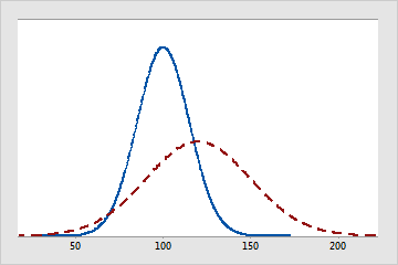
The solid line represents a normal distribution with a mean of 100 and a standard deviation of 15. The dashed line is also a normal distribution, but it has a mean of 120 and a standard deviation of 30.
About parameter estimates (also called sample statistics)
Parameters are descriptive measures of an entire population. However, their values are usually unknown because it is infeasible to measure an entire population. Because of this, you can take a random sample from the population to obtain parameter estimates. One goal of statistical analyses is to obtain estimates of the population parameters along with the amount of error associated with these estimates. These estimates are also known as sample statistics.
- Point estimates are the single, most likely value of a parameter. For example, the point estimate of population mean (the parameter) is the sample mean (the parameter estimate).
- Confidence intervals are a range of values likely to contain the population parameter.
For an example of parameter estimates, suppose you work for a spark plug manufacturer that is studying a problem in their spark plug gap. It would be too costly to measure every single spark plug that is made. Instead, you randomly sample 100 spark plugs and measure the gap in millimeters. The mean of the sample is 9.2. This is the point estimate for the population mean (μ). You also create a 95% confidence interval for μ which is (8.8, 9.6). This means that you can be 95% confident that the true value of the average gap for all the spark plugs is between 8.8 and 9.6.
About sampling distributions
| Pumpkin | 1 | 2 | 3 | 4 | 5 | 6 |
| Weight | 19 | 14 | 15 | 12 | 16 | 17 |
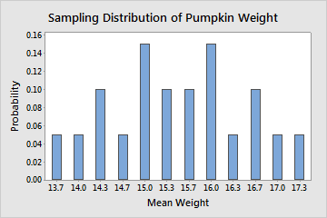
Even though the entire population is known, for illustrative purposes, we take all possible random samples of the population that contain 3 pumpkins (20 random samples). Then, we calculate the mean of each sample. The sampling distribution for the sample mean is described by all the sample means for every possible random sample of 3 pumpkins, which is shown in the following table.
| Sample | Weights | Mean Weight | Probability |
|---|---|---|---|
| 2, 3, 4 | 14, 15, 12 | 13.7 | 1/20 |
| 2, 4, 5 | 14, 12, 16 | 14 | 1/20 |
| 2, 4, 6 | 14, 12, 17 | 14.3 | 2/20 |
| 3, 4, 5 | 15, 12, 16 | ||
| 3, 4, 6 | 15, 12, 17 | 14.7 | 1/20 |
| 1, 2, 4 | 19, 14, 12 | 15 | 3/20 |
| 2, 3, 5 | 14, 15, 16 | ||
| 4, 5, 6 | 12, 16, 17 | ||
| 2, 3, 6 | 14, 15, 17 | 15.3 | 2/20 |
| 1, 3, 4 | 19, 15, 12 | ||
| 1, 4, 5 | 19, 12, 16 | 15.7 | 2/20 |
| 2, 5, 6 | 14, 16, 17 | ||
| 1, 2, 3 | 19, 14, 15 | 16 | 3/20 |
| 3, 5, 6 | 15, 16, 17 | ||
| 1, 4, 6 | 19, 12, 17 | ||
| 1, 2, 5 | 19, 14, 16 | 16.3 | 1/20 |
| 1, 2, 6 | 19, 14, 17 | 16.7 | 2/20 |
| 1, 3, 5 | 19, 15, 16 | ||
| 1, 3, 6 | 19, 15, 17 | 17 | 1/20 |
| 1, 5, 6 | 19, 16, 17 | 17.3 | 1/20 |
In practice, it is prohibitive and unfeasible to tabulate the distribution of the sampling distribution like in the above illustrative example. Even in the best case scenario where you know the parent population of your samples, you may not be able to determine the exact sampling distribution of the sample statistic of interest. However, in some cases you may be able to approximate the sampling distribution of the sample statistic. For example, if you sample from the normal population then the sample mean has exactly the normal distribution.
But if you sample from a population other than normal population, you may not be able to determine the exact distribution of the sample mean. However, because of the central limit theorem, the sample mean is approximately distributed as normal, provided your samples are large enough. Then, if the population is unknown and your samples are large enough you might be able to say, for example, that there is an approximate 85% certainty that the sample mean is within a certain number of standard deviations of the population mean.