In This Topic
Select the model
A quality engineer for a drug manufacturer wants to determine the shelf life for a medication. The concentration of the active ingredient in the medication decreases over time. The engineer wants to determine when the concentration reaches 90% of the intended concentration. The engineer randomly selects 8 batches of medication from a larger population of possible batches and tests one sample from each batch at nine different times.
To estimate the shelf life, the engineer does a stability study. Because the batches are a random sample from a larger population of possible batches, batch is a random factor instead of a fixed factor.
- Open the sample data ShelfLifeRandomBatches.MWX.
- Choose .
- In Response, enter Drug%.
- In Time, enter Month.
- In Batch, enter Batch.
- In Lower spec, enter 90.
- Click Options.
- In the drop-down list, select Batch is a random factor.
- Click OK and then click Graphs.
- Under Residuals Plots, choose Four in one.
- Click OK in each dialog box.
Interpret the results
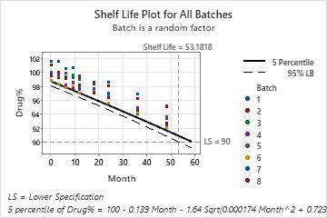
The p-value that compares the models with and without the Month by Batch interaction is 0.059. Because the p-value is less than the significance level of 0.25, the analysis uses the model with the Month by Batch interaction. The shelf life, which is approximately 53 months, is an estimate of the how long the engineer can be 95% confident that 95% of the drug is above the lower specification limit. The estimate applies to any batch that the engineer randomly selects from the process.
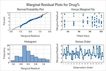
The marginal residuals may not follow a normal distribution with constant variance. The points on the normal probability plot do not follow the line well. One reason for the nonnormal behavior of the marginal residuals is that, when the final model includes the batch by time interaction, the variance of the marginal residuals depends on the time variable and may not be constant. You can use the conditional residuals to check the normality of the error term in the model.
Model Selection with α = 0.25
| Model | -2 LogLikelihood | Difference | P-Value |
|---|---|---|---|
| Month Batch Month*Batch | 128.599 | ||
| Month Batch | 133.424 | 4.82476 | 0.059 |
Variance Components
| Source | Var | % of Total | SE Var | Z-Value | P-Value |
|---|---|---|---|---|---|
| Batch | 0.527409 | 72.91% | 0.303853 | 1.735739 | 0.041 |
| Month*Batch | 0.000174 | 0.02% | 0.000142 | 1.224102 | 0.110 |
| Error | 0.195739 | 27.06% | 0.036752 | 5.325932 | 0.000 |
| Total | 0.723322 |
Model Summary
| S | R-sq | R-sq(adj) |
|---|---|---|
| 0.442424 | 96.91% | 96.87% |
Coefficients
| Term | Coef | SE Coef | DF | T-Value | P-Value |
|---|---|---|---|---|---|
| Constant | 100.060247 | 0.268706 | 7.22 | 372.378347 | 0.000 |
| Month | -0.138766 | 0.005794 | 7.22 | -23.950196 | 0.000 |
Random Effect Predictions
| Term | BLUP | StDev | DF | T-Value | P-Value |
|---|---|---|---|---|---|
| Batch | |||||
| 1 | 1.359433 | 0.313988 | 12.45 | 4.329567 | 0.001 |
| 2 | 0.395375 | 0.313988 | 12.45 | 1.259203 | 0.231 |
| 3 | 0.109151 | 0.313988 | 12.45 | 0.347629 | 0.734 |
| 4 | -0.409322 | 0.313988 | 12.45 | -1.303623 | 0.216 |
| 5 | -0.135643 | 0.313988 | 12.45 | -0.432001 | 0.673 |
| 6 | -1.064736 | 0.313988 | 12.45 | -3.391006 | 0.005 |
| 7 | 0.049420 | 0.313988 | 12.45 | 0.157394 | 0.877 |
| 8 | -0.303678 | 0.313988 | 12.45 | -0.967164 | 0.352 |
| Month*Batch | |||||
| 1 | 0.006281 | 0.008581 | 10.49 | 0.731925 | 0.480 |
| 2 | 0.019905 | 0.008581 | 10.49 | 2.319537 | 0.042 |
| 3 | -0.013831 | 0.008581 | 10.49 | -1.611742 | 0.137 |
| 4 | 0.003468 | 0.008581 | 10.49 | 0.404173 | 0.694 |
| 5 | 0.001240 | 0.008581 | 10.49 | 0.144455 | 0.888 |
| 6 | 0.000276 | 0.008581 | 10.49 | 0.032144 | 0.975 |
| 7 | -0.010961 | 0.008581 | 10.49 | -1.277272 | 0.229 |
| 8 | -0.006378 | 0.008581 | 10.49 | -0.743220 | 0.474 |
Marginal Fits and Diagnostics for Unusual Observations
| Obs | Drug% | Fit | DF | Resid | Std Resid | |
|---|---|---|---|---|---|---|
| 10 | 101.564000 | 99.643950 | 7.04368 | 1.920050 | 2.375254 | R |
| 31 | 100.618000 | 98.811354 | 7.05273 | 1.806646 | 2.213787 | R |
| 55 | 98.481000 | 96.729866 | 8.87383 | 1.751134 | 2.033482 | R |
Shelf Life Estimation
Shelf life = time period in which you can be 95% confident that at least 95% of response is
above lower spec limit
Shelf life for all batches = 53.1818
Check the conditional residuals
- Choose .
- Click Graphs.
- In Residuals for plots, select Conditional regular.
- Click OK in each dialog box.
Interpret the results
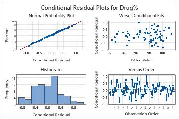
In these results, the conditional residuals appear to follow a normal distribution. The full model appears to fit the data well.