A healthcare provider operates a facility that provides substance abuse treatment services. One of the services at the facility is an outpatient detoxification program where a regular course of treatment can last from 1 to 30 days. A team responsible for projecting staffing and supplies wants to study whether they can make better predictions about the length of time a patient uses services based on information that they can collect about the patient when the patient enters the program. These variables include demographic information and variables about the patient's substance abuse.
First, the team considers a traditional regression analysis in Minitab. Because of the missing value pattern in their data, the analysis omits over 70% of the data. The omission of such a large percentage of data implies that a lot of information is lost. The analytical results from the cases without any missing data can be very different from the results using the entire data set. Because CART® Regression automatically handles missing values in predictor variables, the team decides to use CART® Regression to further evaluate their data.
- Open the sample data set LengthOfService.MWX.
- Choose .
- In Response, enter Length of Service.
- In Continuous predictors, enter Age at Admission-Years of Education.
- In Categorical predictors, enter Other Stimulant Use-DSM Diagnosis.
- Click Validation.
- In Validation method, select K-fold cross-validation.
- Select Assign rows of each fold by ID column.
- In ID column, enter Fold.
- Click OK in each dialog box.
Interpret the results
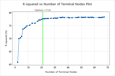
By default, Minitab displays the smallest tree that has an R2 value within 1 standard error of the tree with the maximum R2 value. Because the healthcare team uses k-fold validation, the criterion is the maximum k-fold R2 value. This tree has 21 terminal nodes.
Select an alternative tree
- In the output, click Select Alternative Tree
- In the plot, select the 17-node tree.
- Click Create Tree.
Interpret the results
The researchers look at the plot of the R2 statistic from the cross-validation and the number of terminal nodes. Because the tree with 17 nodes has an R2 statistic close to the largest values on the plot, the results for the rest of the output are for the tree with 17 nodes.
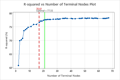
The researchers look first at the model summary to evaluate the performance of the smaller tree. The values for the training and test statistics are close together, so the tree does not seem overfit. The R2 statistic is nearly as high as the 21-node tree, so the researchers decide to use the tree with 17 nodes to explore the relationships between the predictor variables and the response values.
Method
| Node splitting | Least squared error |
|---|---|
| Optimal tree | Within 2.5 standard error of maximum R-squared |
| Model validation | Cross-validation with rows defined by Fold |
| Rows used | 4453 |
Response Information
| Mean | StDev | Minimum | Q1 | Median | Q3 | Maximum |
|---|---|---|---|---|---|---|
| 17.5960 | 9.29097 | 1 | 10 | 18 | 26 | 30 |
Model Summary
| Total predictors | 44 |
|---|---|
| Important predictors | 33 |
| Number of terminal nodes | 17 |
| Minimum terminal node size | 49 |
| Statistics | Training | Test |
|---|---|---|
| R-squared | 77.99% | 76.61% |
| Root mean squared error (RMSE) | 4.3585 | 4.4932 |
| Mean squared error (MSE) | 18.9967 | 20.1887 |
| Mean absolute deviation (MAD) | 3.4070 | 3.5226 |
| Mean absolute percent error (MAPE) | 0.6535 | 0.6674 |
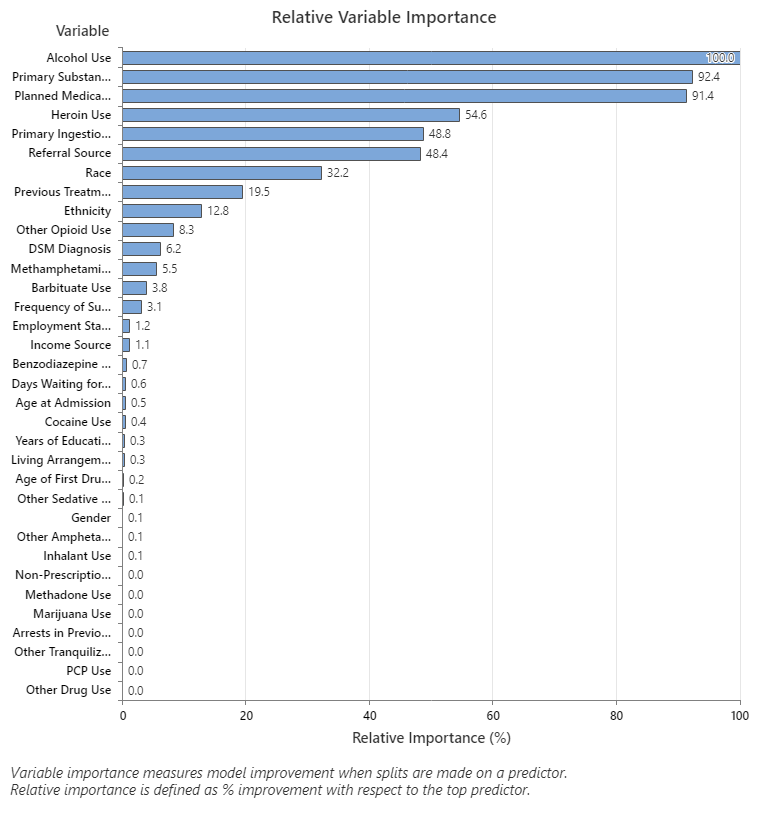
- Primary Substance of Abuse and Planned Medication Therapy are about 92% as important as Alcohol Use.
- Heroin Use is about 55% as important as Alcohol Use.
- Primary Ingestion Route of Sub and Referral Source are about 48% as important as Alcohol Use.
Although these results include 33 variables with positive importance, the relative rankings provide information about how many variables to control or monitor for a certain application. Steep drops in the relative importance values from one variable to the next variable can guide decisions about which variables to control or monitor. For example, in these data, the three most important variables have importance values that are relatively close together before a drop of almost 40% in relative importance to the next variable. Similarly, three variables have similar importance values near 50%. You can remove variables from different groups and redo the analysis to evaluate how variables in various groups affect the prediction accuracy values in the model summary table.
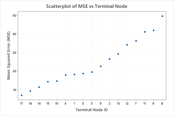
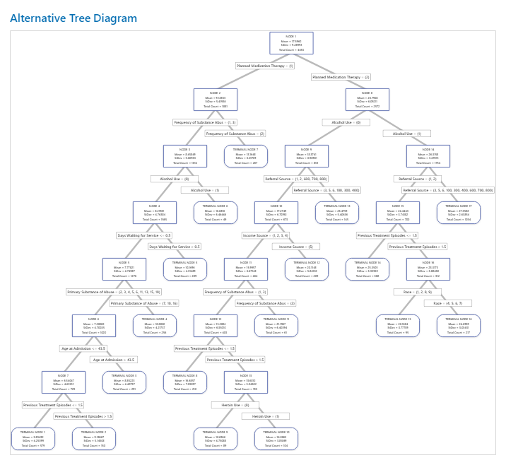
For an analysis with k-fold cross-validation, the tree diagram shows all 4453 cases from the full data set. You can toggle views of the tree between the detailed and node split view. The table of fits and error statistics and the criteria for classifying subjects give additional information about the terminal nodes.
- Node 2 includes the cases where Planned Medication Therapy = 1. This node has 1881 cases. The mean for the node is less than the overall mean. The standard deviation for Node 2 is about 5.4, which is less than the overall standard deviation because a split yields more pure nodes.
- Node 8 includes the cases where Planned Medication Therapy = 2. This node has 2572 cases. The mean for the node is more than the overall mean. The standard deviation for Node 8 is about 6.1, which is also less than the overall standard deviation.
Then, Node 2 splits by Frequency of Substance Abuse and Node 8 splits by the Alcohol Use. Terminal Node 17 has the cases for Planned Medication Therapy = 2, Alcohol Use = 1, and Referral Source = 3, 5, 6, 100, 300, 400, 600, 700, or 800. The researchers note that Terminal Node 17 has the highest mean, the smallest standard deviation, and the most cases.
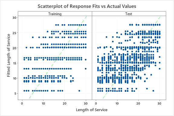
The results include a scatterplot of the fitted response values and the actual response values. The points for the training data set and the test data set show similar patterns. This similarity suggests that the performance of the tree on new data is close to the performance of the tree on the training data.
- Planned Medication Therapy = {2}
- Alcohol Use = {0}
- Referral Source = {1, 2, 600, 700, 800}
- Income Source = {1, 2, 3, 4}
- Frequency of Substance Abuse = {1, 3}
- Previous Treatment Episodes <= 1.5
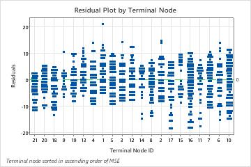
The plot of the residuals by terminal node shows that the fit is too large for a small cluster of the patients in Terminal Node 8. The analysts consider an investigation into why some of these patients use services for less time than a typical patient in their group. For example, if these patients are in a different geographic location from the other patients in the terminal node, then different government and insurance regulations could affect how long they use services.
The plot of the residuals by terminal node shows other cases where analysts can choose to investigate clusters or outliers. For example, in these data, there is one residual that appears much larger than the others in Terminal Node 1 and in Terminal Node 7. The analysts decide to investigate the reason that these patients used services for longer than other patients in their terminal node.
Because the test R2 value leaves room for improvement and the residual plots show cases that the tree does not fit well, the researchers consider whether to use a TreeNet® Regression or a Random Forests® Regression to try to improve the fit.