In This Topic
- Adjusted Blaker exact confidence interval and test methods
- Clopper-Pearson exact confidence interval method
- Test that corresponds to the Clopper-Pearson exact confidence interval
- Wilson-score confidence interval method
- Score test
- Agresti-Coull confidence interval and test methods
- Confidence interval for Wald normal approximation (Web app)
Adjusted Blaker exact confidence interval and test methods
The adjusted Blaker exact method produces two-sided confidence intervals for the proportion of events and produces p-values for the alternative hypothesis of p ≠ p0. Blaker12 provides an exact, two-sided confidence interval by inverting the p-value function of an exact test. The Clopper-Pearson intervals are wider and always contain the Blaker confidence intervals. Intervals from the Blaker exact method are nested. This property means that confidence intervals with higher confidence levels contain confidence intervals with lower confidence levels. For example, an exact, two-sided Blaker 95% confidence interval contains the corresponding 90% confidence interval.
Blaker's original exact method has 2 limitations. One limitation is that the numerical algorithm to calculate the confidence intervals is slow, particularly when the sample size is large. Another limitation is that for some data, the original Blaker exact method produces an interval that covers a hypothesized proportion when the p-value is less than the significance level that corresponds to the confidence level. The limitation also arises when the confidence interval does not contain a hypothesized proportion when the p-value is greater than the significance level that corresponds to the confidence level.
To overcome these limitations, the analysis in Minitab Statistical Software produces the confidence interval and p-value using the algorithm from Klaschka and Reiczigel.3 The name of this method is the adjusted Blaker exact method. This numerical algorithm is faster to calculate and produces confidence intervals and tests that agree in general. The adjusted Blaker confidence intervals are also exact and nested.
For an alternative hypothesis with less than or with greater than, the analysis uses the Clopper-Pearson exact method.
Clopper-Pearson exact confidence interval method
The interval (PL, PU) is a two-sided, 100(1 – α)% confidence interval of p. When the sample has no events, then the lower limit is 0. When the sample has events only, then the upper limit is 1.
Lower limit
Formula
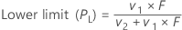
Notation
| Term | Description |
|---|---|
| v1 | 2x |
| v2 | 2(n – x + 1) |
| x | number of events |
| n | number of trials |
| F | lower α/2 point of F distribution with v1 and v2 degrees of freedom |
Upper limit
Formula
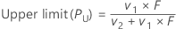
Notation
| Term | Description |
|---|---|
| v1 | 2(x + 1) |
| v2 | 2(n – x) |
| x | number of events |
| n | number of trials |
| F | upper α/2 point of F distribution with v1 and v2 degrees of freedom |
Test that corresponds to the Clopper-Pearson exact confidence interval
Formula
- Ha: p ≠ p0
- p-value =

- Ha: p > p0
- p-value = P{ X ≥ x | p = po}
- Ha: p < p0
- p-value = P{ X ≤ x | p = po}
Notation
| Term | Description |
|---|---|
| p0 | hypothesized proportion |
| n | number of trials |
| p | probability of an event |
| x | number of events |
Wilson-score confidence interval method
Wilson4 inverts the score test to obtain confidence intervals that Minitab Statistical Software names Wilson-score confidence intervals. Wilson-score intervals have two forms, one without a continuity correction and one with a continuity correction. The coverage of the intervals without the correction is sometimes below the nominal confidence level. The actual confidence level of the intervals with the correction is at least the nominal confidence level. For both methods when the sample has no events, then the lower limit is 0. When the sample has events only, then the upper limit is 1.
Intervals without the continuity correction
The two-sided, 100(1 – α)% confidence interval has the following formula:

Intervals with the continuity correction
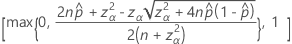
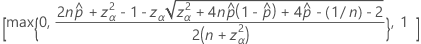
The lower bound of the two-sided 100(1 – α)% interval has the following formula:
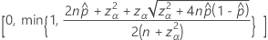
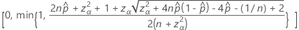
The upper bound of the two-sided, 100(1 – α)% interval has the following formula:

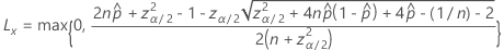
The one-sided, 100(1 – α)% lower limit has the following formula:
The one-sided, 100(1 – α)% upper limit has the following formula:
Notation
| Term | Description |
|---|---|
 | observed probability,  = x / n = x / n |
| x | number of events |
| n | number of trials |
| zγ | the upper percentile point of the standard normal distribution at γ |
| α | 1 – confidence level/100 |
Score test
Method without the continuity correction
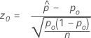
The test that corresponds to the Wilson-score confidence interval and the normal approximation method (Web app) is the well-known score test. The score test statistic has the following equation:
- Ha: p ≠ p0
- p-value =

- Ha: p > p0
- p-value =

- Ha: p < p0
- p-value =

Method with the continuity correction
The test statistic and p-value for the procedure with a continuity correction depend on the alternative hypothesis.
- Ha: p ≠ p0
-
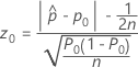
- p-value =

- Ha: p > p0
-
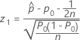
- p-value =

- Ha: p < p0
-
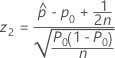
- p-value =

Notation
| Term | Description |
|---|---|
 | observed probability, x/n |
| x | number of events |
| n | number of trials |
| p0 | hypothesized proportion |
 | cumulative distribution function of the standard normal distribution at y |
Agresti-Coull confidence interval and test methods
Confidence interval
Agresti and Coull5 provide an adjustment to the Wald method for confidence intervals that improves the coverage properties. For a two-sided, 95% confidence interval, the adjustment approximately adds 2 events and 2 non-events, then calculates the confidence intervals from the formulas for the Wald confidence interval formulas. When the sample has no events, then the lower limit is 0. When the sample has events only, then the upper limit is 1.
The two-sided, 100(1 – α)% interval has the following formula:

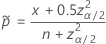
and

The one-sided, 100(1 – α)% lower limit has the following formula:

The one-sided, 100(1 – α)% upper limit has the following formula:
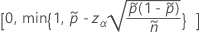
For the one-sided limits, use  in the definition of
  and
and  :
:


Test that corresponds to the Agresti-Coull interval
The analysis calculates the p-value for the test by inverting the confidence interval procedure.
Notation
| Term | Description |
|---|---|
| x | number of events |
| n | number of trials |
| zγ | the upper percentile point of the standard normal distribution at γ |
| α | 1 – confidence level/100 |
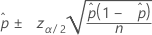
Confidence interval for Wald normal approximation (Web app)
Formula
Notation
| Term | Description |
|---|---|
 | observed probability,  = x / n = x / n |
| x | observed number of events in n trials |
| n | number of trials |
| zα/2 | inverse cumulative probability of the standard normal distribution at 1–α/2 |
| α | 1 – confidence level/100 |