In This Topic
Histogram
A histogram divides sample values into many intervals and represents the frequency of data values in each interval with a bar.
Interpretation
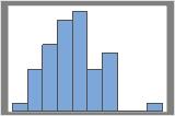
50 resamples
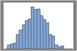
1000 resamples
The distribution is usually easier to determine with more resamples. For example, in these data, the distribution is ambiguous for 50 resamples. With 1000 resamples, the shape looks approximately normal.
In this histogram, the bootstrap distribution appears to be normal.
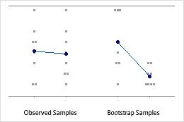
Individual value plot
An individual value plot displays the individual values in the sample. Each circle represents one observation. An individual value plot is especially useful when you have relatively few observations and when you also need to assess the effect of each observation.
Note
Minitab displays an individual value plot only when you take only one resample. Minitab displays both the original data and the resample data.
Interpretation
Sample size of 8
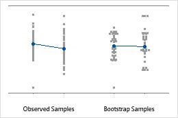
Sample size of 50
Number of Resamples
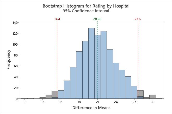
The number of resamples is the number of times Minitab takes a random sample with replacement from your original data set. Usually, a large number of resamples works best. The sample size for each resample is equal to the sample size of the original data set. The number of resamples equals the number of observations on the histogram.
Average
The average is the sum of all the differences in means of the bootstrapping sample divided by the number of resamples.
Interpretation
Minitab displays two different values for the difference in means, the difference of the observed samples and the difference of the bootstrap distribution (Average). Both these values are an estimate of the difference in population means and will usually be similar. If there is a large difference between these two values, you should increase the sample size of your original sample.
Because the average is based on sample data and not the entire population, it is unlikely that the average equals the difference in population means. To better estimate the difference in population means, use the confidence interval.
StDev (bootstrap sample)
The standard deviation is the most common measure of dispersion, or how spread out the data are about the mean. The symbol σ (sigma) is often used to represent the standard deviation of a population, while s is used to represent the standard deviation of a sample. Variation that is random or natural to a process is often referred to as noise. Because the standard deviation is in the same units as the data, it is usually easier to interpret than the variance.
The standard deviation of the bootstrap samples (also known as the bootstrap standard error) is an estimate of the standard deviation of the sampling distribution of the difference in means.
Interpretation
Use the standard deviation to determine how spread out the differences from the bootstrap sample are from the overall mean of the differences. A higher standard deviation value indicates greater spread in the differences. A good rule of thumb for a normal distribution is that approximately 68% of the values fall within one standard deviation of the overall mean of the differences, 95% of the values fall within two standard deviations, and 99.7% of the values fall within three standard deviations.
Use the standard deviation of the bootstrap samples to determine how precisely the differences from the bootstrap sample estimate the population difference in means. A smaller value indicates a more precise estimate of the population difference. Usually, a larger standard deviation results in a larger bootstrap standard error and a less precise estimate of the population difference. A larger sample size results in a smaller bootstrap standard error and a more precise estimate of the population difference.
Confidence interval (CI) and bounds
Confidence intervals are based on the sampling distribution of a statistic. If a statistic has no bias as an estimator of a parameter, its sampling distribution is centered at the true value of the parameter. A bootstrapping distribution approximates the sampling distribution of the statistic. Therefore, the middle 95% of values from the bootstrapping distribution provide a 95% confidence interval for the parameter. The confidence interval helps you assess the practical significance of your estimate for the population parameter. Use your specialized knowledge to determine whether the confidence interval includes values that have practical significance for your situation.
Note
Minitab does not calculate the confidence interval when the number of resamples is too small to obtain an accurate confidence interval.
Observed Samples
| Hospital | N | Mean | StDev | Variance | Minimum | Median | Maximum |
|---|---|---|---|---|---|---|---|
| A | 20 | 80.30 | 8.18 | 66.96 | 62.00 | 79.00 | 98.00 |
| B | 20 | 59.30 | 12.43 | 154.54 | 35.00 | 58.50 | 89.00 |
Difference in Observed Means
| Mean of A - Mean of B = 21 |
|---|
Bootstrap Samples for Difference in Means
| Number of Resamples | Average | StDev | 95% CI for Difference |
|---|---|---|---|
| 1000 | 20.960 | 3.279 | (14.400, 27.600) |
In these results, the estimate for the population difference is 20.96. You can be 95% confident that the population difference is between 14.4 and 27.6.