What is regression analysis?
A regression analysis generates an equation to describe the statistical relationship between one or more predictors and the response variable and to predict new observations. Linear regression usually uses the ordinary least squares estimation method which derives the equation by minimizing the sum of the squared residuals.
For example, you work for a potato chip company that is analyzing factors that affect the percentage of crumbled potato chips per container before shipping (response variable). You are conducting the regression analysis and include the percentage of potato relative to other ingredients and the cooking temperature (Celsius) as your two predictors. The following is a table of the results.
Regression Analysis: Broken Chips versus Potato Percentage, Cooking temperature
- For each 1 degree Celsius increase in cooking temperature, the percentage of broken chips is expected to increase by 0.022%.
- To predict the percentage of broken chips for settings of 0.5 (50%) potato and a cooking temperature of 175 °C, you calculate an expected value of 7.7% broken potato chips: 4.251 - 0.909 * 0.5 + 0.2231 * 175 = 7.70075.
- The sign of each coefficient indicates the direction of the relationship.
- Coefficients represent the mean change in the response for one unit of change in the predictor while holding other predictors in the model constant.
- The P-value for each coefficient tests the null hypothesis that the coefficient is equal to zero (no effect). Therefore, low p-values indicate the predictor is a meaningful addition to your model.
- The equation predicts new observations given specified predictor values.
Note
Models with one predictor are referred to as simple regression. Models with more than one predictor are known as multiple linear regression.
What is simple linear regression?
Simple linear regression examines the linear relationship between two continuous variables: one response (y) and one predictor (x). When the two variables are related, it is possible to predict a response value from a predictor value with better than chance accuracy.
- Examine how the response variable changes as the predictor variable changes.
- Predict the value of a response variable (y) for any predictor variable (x).
What is multiple linear regression?
Multiple linear regression examines the linear relationships between one continuous response and two or more predictors.
If the number of predictors is large, then before fitting a regression model with all the predictors, you should use stepwise or best subsets model-selection techniques to screen out predictors not associated with the responses.
What is ordinary least squares regression?
In ordinary least squares (OLS) regression, the estimated equation is calculated by determining the equation that minimizes the sum of the squared distances between the sample's data points and the values predicted by the equation.
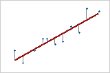
Response vs. Predictor
With one predictor (simple linear regression), the sum of the squared distances from each point to the line are as small as possible.
Assumptions that should be met for OLS regression
- The regression model is linear in the coefficients. Least squares can model curvature by transforming the variables (instead of the coefficients). You must specify the correct functional form in order to model any curvature.
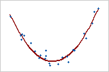
Quadratic Model
Here, the predictor variable, X, is squared in order to model the curvature. Y = bo + b1X + b2X2
- Residuals have a mean of zero. Inclusion of a constant in the model will force the mean to equal zero.
- All predictors are uncorrelated with the residuals.
- Residuals are not correlated with each other (serial correlation).
- Residuals have a constant variance.
- No predictor variable is perfectly correlated (r=1) with a different predictor variable. It is best to avoid imperfectly high correlations (multicollinearity) as well.
- Residuals are normally distributed.
Because OLS regression will provide the best estimates only when all the assumptions are met, it is very important to test them. Common approaches include examining residual plots, using lack-of-fit tests, and viewing the correlation between predictors using the Variance Inflation Factor (VIF).