In This Topic
Exponential family and link functions
The extension of the classical linear models to generalized linear models has two parts: a distribution from the exponential family and a link function.
The exponential family
The first part extends the linear model to response variables that are members of a large family of distributions called the exponential family. Members of the exponential family of distributions have probability distribution functions for an observed response in this general form:
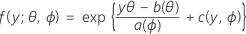
where a(∙), b(∙), and c(∙) depend on the distribution of the response variable. The parameter θ is a location parameter that is often called the canonical parameter, and ϕ is called the dispersion parameter. The function a(ϕ) is usually of the form a(ϕ)= ϕ/ ω, where ω is a known constant or weight that may vary from one observation to another. (In Minitab, when weights are given the function a(ϕ), is adjusted accordingly.)
Members of the exponential family can be discrete distributions or continuous distributions. Examples of continuous distributions that are members of the exponential family are the normal and the gamma distributions. Examples of discrete distributions that are members of the exponential family are the binomial and the Poisson distributions. The following table gives the characteristics of some of these distributions.
| Distribution | ϕ | b(θ) | a(φ) | c(y, ϕ) |
| Normal | σ2 | θ2/2 | φω | 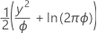 |
| Binomial | 1 |  |
φ/ω | -ln(y!) |
| Poisson | 1 | exp(θ) | φ/ω |  |
The link function
The second part is the link function. The link function relates the mean of the response in the ith observation to a linear predictor in this form:

The classical linear model is a special case of this general formulation where the link function is the identity function.
The choice of the link function in the second part depends upon the specific distribution of the exponential family of the first part. In particular, each distribution in the exponential family has a special link function called the canonical link function. This link function satisfies the equation g (μi) = Xi'β= θ, where θ is the canonical parameter. The canonical link function results in some desirable statistical properties of the model. Goodness-of-fit statistics can be used to compare fits using different link functions. Certain link functions may be used for historical reasons or because they have a special meaning in a discipline. For example, an advantage of the logit link function is that it provides an estimate of the odds ratios. Another example is that the normit link function assumes that there is an underlying variable that follows a normal distribution that is classified into binary categories.
Minitab provides three link functions for each class of models. The different link functions make it possible to find models that adequately fit a wider variety of data.
For binomial models, the link functions are logit, normit (also called probit), and gompit (also called complementary log-log). These are the inverse of the standard cumulative logistic distribution function (logit), the inverse of the standard cumulative normal distribution function (normit), and the inverse of the Gompertz distribution function (gompit). The logit is the canonical link function for binomial models, thus the logit is the default link function.
For Poisson models, the link functions are the natural log, the square root, and the identity. The natural log is the canonical link function for Poisson models, thus the natural log is the default link function.
The link functions are summarized below:
| Model | Name | Link Function, g(μi) |
| Binomial | logit |  |
| Binomial | normit (probit) |  |
| Binomial | gompit (complementary log-log) |  |
| Poisson | natural log |  |
| Poisson | square root |  |
| Poisson | identity |  |
Notation
| Term | Description |
|---|---|
| μi | the mean response of the ith row |
| g(μi) | the link function |
| X | the vector of predictor variables |
| β | the vector of coefficients associated with the predictors |
 | the inverse cumulative distribution function of the normal distribution |
Factor/covariate pattern
Describes a single set of factor/covariate values in a data set. Minitab calculates event probabilities, residuals, and other diagnostic measures for each factor/covariate pattern.
For example, if a data set includes the factors gender and race and the covariate age, the combination of these predictors may contain as many different covariate patterns as subjects. If a data set only includes the factors race and sex, each coded at two levels, there are only four possible factor/covariate patterns. If you enter your data as frequencies, or as successes, trials, or failures, each row contains one factor/covariate pattern.
Internal weights for Fit Binary Logistic Model
Formula
- Logit

- Normit

- Gompit

Notation
| Term | Description |
|---|---|
| mi | the number of trials for the ith row |
 | the predicted probability for the design point in a binary logistic model |
| yi | the number of events for the ith row |
 | the inverse cumulative distribution function of the standard normal distribution for the predicted probability in a binary logistic model |
How Minitab removes highly correlated predictors from the regression equation in Fit Binary Logistic Model
Let rij be the element in the current swept matrix associated with Xi and Xj.
Variables are entered or removed one at a time. Xk is eligible for entry if it is an independent variable not currently in the model with rkk ≥ 1 (tolerance with a default of 0.0001) and also for each variable Xj that is currently in the model,

- Minitab performs the SWEEP method on the correlation matrix, R, treating X1 … Xp as if they are random variables.
- For any continuous predictor, Minitab compares the element rkk with the tolerance; rkk ≥ tolerance, where k = 1 to p.
- For each variable Xj currently in the model, Minitab checks that (rjj – rjk * (rkj / rkk)) * tolerance ≤ 1.
Note
Where rkk, rjk, rjj are the corresponding diagonal and off diagonal elements for Xj and Xk variables after k step SWEEP operations.
- Otherwise, the predictor fails the test and is removed from the model.
Note
The default tolerance value is 8.8e–12.
Note
You can use the TOLERANCE subcommand with the GZLM session command to force Minitab to keep a predictor in the model that is highly correlated with a different predictor. However, lowering the tolerance can be dangerous, possibly producing numerically inaccurate results.