In This Topic
Step 1: Examine the similarity and distance levels
At each step in the amalgamation process, view the clusters that are formed and examine their similarity and distance levels. The higher the similarity level, the more similar the observations are in each cluster. The lower the distance level, the closer the observations are in each cluster.
Ideally, the clusters should have a relatively high similarity level and a relatively low distance level. However, you must balance that goal with having a reasonable and practical number of clusters.
Amalgamation Steps
| Step | Number of clusters | Similarity level | Distance level | Clusters joined | New cluster | Number of obs. in new cluster | |
|---|---|---|---|---|---|---|---|
| 1 | 19 | 96.6005 | 0.16275 | 13 | 16 | 13 | 2 |
| 2 | 18 | 95.4642 | 0.21715 | 17 | 20 | 17 | 2 |
| 3 | 17 | 95.2648 | 0.22669 | 6 | 9 | 6 | 2 |
| 4 | 16 | 92.9178 | 0.33905 | 17 | 18 | 17 | 3 |
| 5 | 15 | 90.5296 | 0.45339 | 11 | 15 | 11 | 2 |
| 6 | 14 | 90.3124 | 0.46378 | 12 | 19 | 12 | 2 |
| 7 | 13 | 88.2431 | 0.56285 | 2 | 14 | 2 | 2 |
| 8 | 12 | 88.2431 | 0.56285 | 5 | 8 | 5 | 2 |
| 9 | 11 | 85.9744 | 0.67146 | 6 | 10 | 6 | 3 |
| 10 | 10 | 83.0639 | 0.81080 | 7 | 13 | 7 | 3 |
| 11 | 9 | 83.0639 | 0.81080 | 1 | 3 | 1 | 2 |
| 12 | 8 | 81.4039 | 0.89027 | 2 | 17 | 2 | 5 |
| 13 | 7 | 79.8185 | 0.96617 | 6 | 11 | 6 | 5 |
| 14 | 6 | 78.7534 | 1.01716 | 4 | 12 | 4 | 3 |
| 15 | 5 | 66.2112 | 1.61760 | 2 | 5 | 2 | 7 |
| 16 | 4 | 62.0036 | 1.81904 | 1 | 6 | 1 | 7 |
| 17 | 3 | 41.0474 | 2.82229 | 1 | 4 | 1 | 10 |
| 18 | 2 | 40.1718 | 2.86421 | 2 | 7 | 2 | 10 |
| 19 | 1 | 0.0000 | 4.78739 | 1 | 2 | 1 | 20 |
Key Results: Similarity level, Distance level
In these results, the data contain a total of 20 observations. In step 1, two clusters (observations 13 and 16 in the worksheet) are joined to form a new cluster. This step creates 19 clusters in the data, with a similarity level of 96.6005 and a distance level of 0.16275. Although the similarity level is high and the distance level is low, the number of clusters is too high to be useful. At each subsequent step, as new clusters are formed, the similarity level decreases and the distance level increases. At the final step, all the observations are joined into a single cluster.
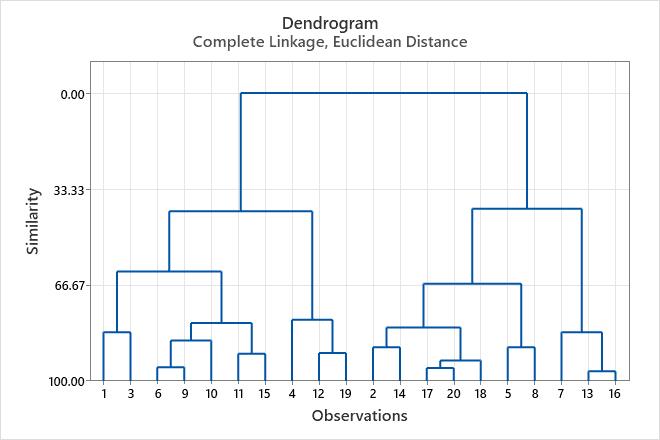
To view the similarity levels in the dendrogram, hold your pointer over a horizontal line in the tree diagram, in Minitab.
Step 2: Determine the final groupings for your data
Use the similarity level for the clusters that are joined at each step to help determine the final groupings for the data. Look for an abrupt change in the similarity level between steps. The step that precedes the abrupt change in similarity may provide a good cut-off point for the final partition. For the final partition, the clusters should have a reasonably high similarity level. You should also use your practical knowledge of the data to determine the final groupings that make the most sense for your application.
For example, the following amalgamation table shows that the similarity level decreases by increments of approximately 3 or less until step 15. The similarity decreases by more than 20 (from 62.0036 to 41.0474) at steps 16 and 17, when the number of clusters changes from 4 to 3. These results indicate that 4 clusters may be sufficient for the final partition. If this grouping makes intuitive sense, then it is probably a good choice.
Amalgamation Steps
| Step | Number of clusters | Similarity level | Distance level | Clusters joined | New cluster | Number of obs. in new cluster | |
|---|---|---|---|---|---|---|---|
| 1 | 19 | 96.6005 | 0.16275 | 13 | 16 | 13 | 2 |
| 2 | 18 | 95.4642 | 0.21715 | 17 | 20 | 17 | 2 |
| 3 | 17 | 95.2648 | 0.22669 | 6 | 9 | 6 | 2 |
| 4 | 16 | 92.9178 | 0.33905 | 17 | 18 | 17 | 3 |
| 5 | 15 | 90.5296 | 0.45339 | 11 | 15 | 11 | 2 |
| 6 | 14 | 90.3124 | 0.46378 | 12 | 19 | 12 | 2 |
| 7 | 13 | 88.2431 | 0.56285 | 2 | 14 | 2 | 2 |
| 8 | 12 | 88.2431 | 0.56285 | 5 | 8 | 5 | 2 |
| 9 | 11 | 85.9744 | 0.67146 | 6 | 10 | 6 | 3 |
| 10 | 10 | 83.0639 | 0.81080 | 7 | 13 | 7 | 3 |
| 11 | 9 | 83.0639 | 0.81080 | 1 | 3 | 1 | 2 |
| 12 | 8 | 81.4039 | 0.89027 | 2 | 17 | 2 | 5 |
| 13 | 7 | 79.8185 | 0.96617 | 6 | 11 | 6 | 5 |
| 14 | 6 | 78.7534 | 1.01716 | 4 | 12 | 4 | 3 |
| 15 | 5 | 66.2112 | 1.61760 | 2 | 5 | 2 | 7 |
| 16 | 4 | 62.0036 | 1.81904 | 1 | 6 | 1 | 7 |
| 17 | 3 | 41.0474 | 2.82229 | 1 | 4 | 1 | 10 |
| 18 | 2 | 40.1718 | 2.86421 | 2 | 7 | 2 | 10 |
| 19 | 1 | 0.0000 | 4.78739 | 1 | 2 | 1 | 20 |
Key Results: Similarity level, Number of clusters
The decision about final grouping is also called cutting the dendrogram. Cutting the dendrogram is similar to drawing a horizontal line across the dendrogram to specify the final grouping. For example, to cut this dendrogram into four clusters, imagine drawing a horizontal line about halfway down the vertical axis, just below the similarity level of approximately 41.
Step 3: Examine the final partition
After you determine the final groupings in step 2, rerun the analysis and specify the number of clusters (or the similarity level) for the final partition. Minitab displays the final partition table, which shows the characteristics of each cluster in the final partition. For example, the average distance from the centroid provides a measure of the variability of the observations within each cluster.
Note
For more information on these statistics, go to Final partition.
Final Partition
| Number of observations | Within cluster sum of squares | Average distance from centroid | Maximum distance from centroid | |
|---|---|---|---|---|
| Cluster1 | 7 | 3.25713 | 0.612540 | 1.12081 |
| Cluster2 | 7 | 2.72247 | 0.581390 | 0.95186 |
| Cluster3 | 3 | 0.55977 | 0.398964 | 0.54907 |
| Cluster4 | 3 | 0.37116 | 0.326533 | 0.48848 |
Cluster Centroids
| Variable | Cluster1 | Cluster2 | Cluster3 | Cluster4 | Grand centroid |
|---|---|---|---|---|---|
| Gender | 0.97468 | -0.97468 | 0.97468 | -0.97468 | -0.0000000 |
| Height | -1.00352 | 1.01283 | -0.37277 | 0.35105 | 0.0000000 |
| Weight | -0.90672 | 0.93927 | -0.86797 | 0.79203 | -0.0000000 |
| Handedness | 0.63808 | 0.63808 | -1.48885 | -1.48885 | 0.0000000 |
Distances Between Cluster Centroids
| Cluster1 | Cluster2 | Cluster3 | Cluster4 | |
|---|---|---|---|---|
| Cluster1 | 0.00000 | 3.35759 | 2.21882 | 3.61171 |
| Cluster2 | 3.35759 | 0.00000 | 3.67557 | 2.23236 |
| Cluster3 | 2.21882 | 3.67557 | 0.00000 | 2.66074 |
| Cluster4 | 3.61171 | 2.23236 | 2.66074 | 0.00000 |
Key Results: Final partition, dendrogram
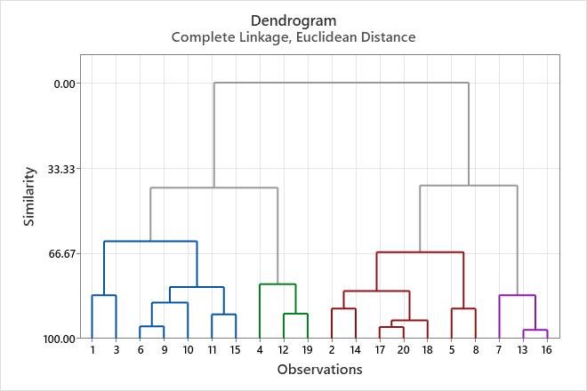
This dendrogram was created using a final partition of 4 clusters, which occurs at a similarity level of approximately 40. The first cluster (far left) is composed of seven observations (the observations in rows 1, 3, 6, 9, 10, 11, and 15 of the worksheet). The second cluster, directly to the right, is composed of 3 observations (the observations in rows 4, 12, and 19 of the worksheet). The third cluster is composed of 7 observations (the observations in rows 2, 14, 17, 20, 18, 5, and 8). The fourth cluster, on the far right, is composed of 3 observations (the observations in rows 7, 13, and 16). If you cut the dendrogram higher, then there would be fewer final clusters, but their similarity level would be lower. If you cut the dendrogram lower, then the similarity level would be higher, but there would be more final clusters.