Exponential distribution
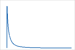
Use the exponential distribution to model the time between events in a continuous Poisson process. It is assumed that independent events occur at a constant rate.
This distribution has a wide range of applications, including reliability analysis of products and systems, queuing theory, and Markov chains.
- How long it takes for electronic components to fail
- The time interval between customers' arrivals at a terminal
- Service time for customers waiting in line
- The time until default on a payment (credit risk modeling)
- Time until a radioactive nucleus decays
For the 1-parameter exponential distribution, the threshold is zero, and the distribution is defined by its scale parameter. For the 1-parameter exponential distribution, the scale parameter equals the mean.
What does memoryless mean?
An important property of the exponential distribution is that it is memoryless. The chance of an event does not depend on past trials. Therefore, the occurrence rate remains constant.
The memoryless property indicates that the remaining life of a component is independent of its current age. For example, random trials of a coin toss demonstrate the memoryless property. A system that has wear and tear, and thus becomes more likely to fail later in its life, is not memoryless.
Gamma distribution
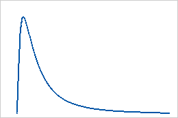
Use the gamma distribution to model positive data values that are skewed to the right and greater than 0. The gamma distribution is commonly used in reliability survival studies. For example, the gamma distribution can describe the time for an electrical component to fail. Most electrical components of a particular type will fail around the same time, but a few will take a long time to fail.
When the shape parameter is an integer, the gamma distribution is sometimes called an Erlang distribution. The Erlang distribution is commonly used in queuing theory applications.
Logistic distribution
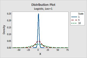
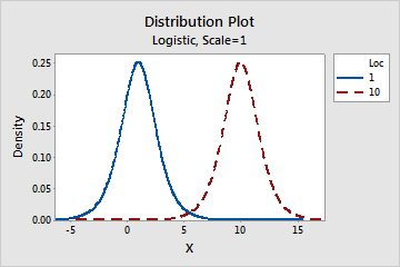
Use the logistic distribution to model data distributions that have longer tails and higher kurtosis than the normal distribution.
- Effect of scale parameter
- The following graph shows the effect of the different values of the scale parameter
on the logistic distribution.
- Effect of location parameter
- The following graph shows the effect of the different values of the location
parameter on the logistic distribution.
Loglogistic distribution
Use the loglogistic distribution when the logarithm of the variable is logistically distributed. For example, the loglogistic distribution is used in growth models and to model binary responses in fields such as biostatistics and economics.
The loglogistic distribution is a continuous distribution that is defined by its scale and location parameters. The 3-parameter loglogistic distribution is defined by its scale, location, and threshold parameters.
The loglogistic distribution is also known as the Fisk distribution.
Lognormal distribution
Use the lognormal distribution if the logarithm of the random variable is normally distributed. Use when random variables are greater than 0. For example, the lognormal distribution is used for reliability analysis and in financial applications, such as modeling stock behavior.
The lognormal distribution is a continuous distribution that is defined by its location and scale parameters. The 3-parameter lognormal distribution is defined by its location, scale, and threshold parameters.
Normal distribution
The normal distribution is a continuous distribution that is specified by the mean (μ) and the standard deviation (σ). The mean is the peak or center of the bell-shaped curve. The standard deviation determines the spread of the distribution.
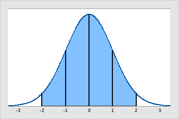
The normal distribution is the most common statistical distribution because approximate normality occurs naturally in many physical, biological, and social measurement situations. Many statistical analyses assume that the data come from approximately normally distributed populations.
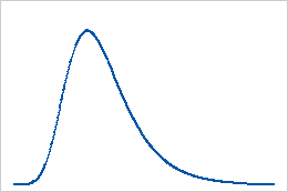
Smallest and largest extreme value distributions
The largest extreme value distribution and the smallest extreme value distribution are closely related. For example, if X has a largest extreme value distribution, then −X has a smallest extreme value distribution, and vice versa.
Smallest extreme value distribution
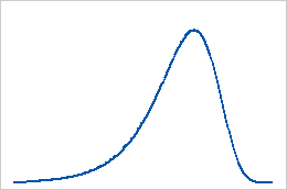
Largest extreme value distribution
Weibull distribution
The Weibull distribution is a versatile distribution that can be used to model a wide range of applications in engineering, medical research, quality control, finance, and climatology. For example, the distribution is frequently used with reliability analyses to model time-to-failure data. The Weibull distribution is also used to model skewed process data in capability analysis.
The Weibull distribution is described by the shape, scale, and threshold parameters, and is also known as the 3-parameter Weibull distribution. The case when the threshold parameter is zero is called the 2-parameter Weibull distribution. The 2-parameter Weibull distribution is defined only for positive variables. A 3-parameter Weibull distribution can work with zeros and negative data, but all data for a 2-parameter Weibull distribution must be greater than zero.
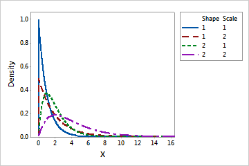
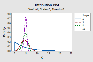
Depending on the values of its parameters, the Weibull distribution can take various forms.
- Effect of the shape parameter
- The shape parameter describes how your data are distributed. A shape of 3 approximates
a normal curve. A low value for shape, say 1, gives a right-skewed curve. A high value
for shape, say 10, gives a left-skewed curve.
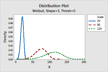
- Effect of the scale parameter
- The scale, or characteristic life, is the 63.2 percentile of the data. The scale
defines the position of the Weibull curve relative to the threshold, which is analogous
to the way the mean defines the position of a normal curve. A scale of 20, for example,
indicates that 63.2% of the equipment will fail in the first 20 hours after the
threshold time.
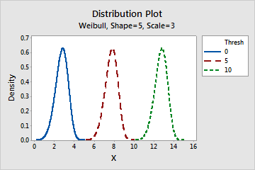
- Effect of the threshold parameter
- The threshold parameter describes the shift of the distribution away from 0. A
negative threshold shifts the distribution to the left, and a positive threshold shifts
the distribution to the right. All data must be greater than the threshold. The
2-parameter Weibull distribution is the same as the 3-parameter Weibull with a threshold
of 0. For example, the 3-parameter Weibull (3,100,50) has the same shape and spread as
the 2-parameter Weibull (3,100), but is shifted 50 units to the right.