An engineer for a golf equipment manufacturer wants to design a new golf ball to maximize ball flight distance. The engineer has identified four control factors (core material, core diameter, number of dimples, and cover thickness) and one noise factor (type of golf club). Each control factor has 2 levels. The noise factor is two types of golf clubs: driver and a 5-iron. The engineer measures flight distance for each club type, and records the data in two noise factor columns in the worksheet.
Because the goal of the experiment is to maximize flight distance, the engineer uses the larger-is-better signal-to-noise ratio (S/N). The engineer also wants to test the interaction between core material and core diameter.
- Open the sample data, GolfBall.MWX.
- Choose .
- In Response data are in, enter Driver and Iron.
- Click Analysis.
- Under Fit linear model for, check Signal to Noise ratios and Means. Click OK.
- Click Terms.
- Move terms A: Material, B: Diameter, C: Dimples, D: Thickness, and AB from Available Terms to Selected Terms. Click OK.
- Click Options.
- Under Signal to Noise Ratio, select Larger is better. Click OK.
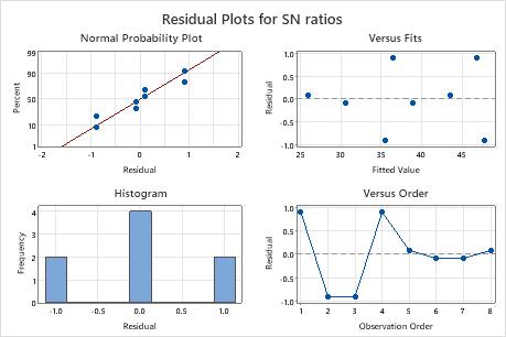
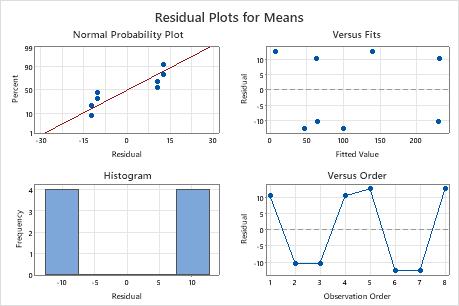
- Click Analysis Graphs, then select Four in one.
- Click OK in each dialog box.
Interpret the results
Minitab provides an estimated regression coefficients table for each response characteristic that you select. In this example, the engineer chose two response characteristics — the signal-to-noise ratio (S/N) and the means. Use the p-values to determine which factors are statistically significant and use the coefficients to determine each factor's relative importance in the model.
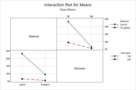
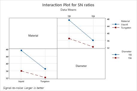
In this example, for S/N ratios, all the factors have a p-value less than 0.05 and are statistically significant at a significance level of 0.05. Frequently, a significance level of 0.10 is used for evaluating terms in a model. The interaction is statistically significant at a significance level of 0.10. For means, core material (p = 0.045) and core diameter (p = 0.024) are statistically significant at a significance level of 0.05, and the interaction of material with diameter (p = 0.06) is statistically significant at a significance level of 0.10. However, because both factors are involved in the interaction, you need to understand the interaction before you can consider the effect of each factor individually.
The absolute value of the coefficient indicates the relative strength of each factor. The factor with the largest coefficient has the largest impact on a given response characteristic. In Taguchi designs, the magnitude of the factor coefficient usually mirrors the factor ranks in the response tables.
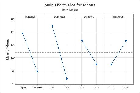
The response tables show the average of each response characteristic for each level of each factor. The tables include ranks based on Delta statistics, which compare the relative magnitude of effects. The Delta statistic is the highest minus the lowest average for each factor. Minitab assigns ranks based on Delta values; rank 1 to the highest Delta value, rank 2 to the second highest, and so on. Use the level averages in the response tables to determine which level of each factor provides the best result.
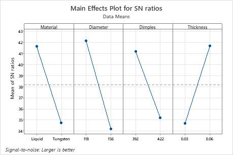
In Taguchi experiments, you always want to maximize the S/N ratio. In this example, the ranks indicate that core diameter (B) has the most influence on both the S/N ratio and the mean. For S/N ratio, cover thickness (D) has the next largest influence, followed by core material (A) and dimples (C). For means, core material (A) has the next largest influence, followed by dimples (C) and cover thickness (D).
- Liquid core (A)
- Core diameter (B) = 118
- Dimples (C) = 392
- Cover thickness (D) = 0.06
To continue this analysis, the engineer can use Predict Taguchi Results to determine the predicted S/N ratios and means at these factor settings. For more information, go to Example of Predict Taguchi Results
Model Summary
| S | R-Sq | R-Sq(adj) |
|---|---|---|
| 1.2793 | 99.21% | 97.23% |
Analysis of Variance for SN ratios
| Source | DF | Seq SS | Adj SS | Adj MS | F | P |
|---|---|---|---|---|---|---|
| Material | 1 | 94.427 | 94.427 | 94.427 | 57.70 | 0.017 |
| Diameter | 1 | 125.917 | 125.917 | 125.917 | 76.94 | 0.013 |
| Dimples | 1 | 71.133 | 71.133 | 71.133 | 43.47 | 0.022 |
| Thickness | 1 | 96.828 | 96.828 | 96.828 | 59.17 | 0.016 |
| Material*Diameter | 1 | 21.504 | 21.504 | 21.504 | 13.14 | 0.068 |
| Residual Error | 2 | 3.273 | 3.273 | 1.637 | ||
| Total | 7 | 413.083 |
Estimated Model Coefficients for Means
| Term | Coef | SE Coef | T | P |
|---|---|---|---|---|
| Constant | 110.40 | 8.098 | 13.634 | 0.005 |
| Material Liquid | 36.86 | 8.098 | 4.552 | 0.045 |
| Diameter 118 | 51.30 | 8.098 | 6.335 | 0.024 |
| Dimples 392 | 23.25 | 8.098 | 2.871 | 0.103 |
| Thicknes 0.03 | -22.84 | 8.098 | -2.820 | 0.106 |
| Material*Diameter Liquid 118 | 31.61 | 8.098 | 3.904 | 0.060 |
Model Summary
| S | R-Sq | R-Sq(adj) |
|---|---|---|
| 22.9035 | 97.88% | 92.58% |
Analysis of Variance for Means
| Source | DF | Seq SS | Adj SS | Adj MS | F | P |
|---|---|---|---|---|---|---|
| Material | 1 | 10871 | 10871 | 10870.8 | 20.72 | 0.045 |
| Diameter | 1 | 21054 | 21054 | 21053.5 | 40.13 | 0.024 |
| Dimples | 1 | 4325 | 4325 | 4324.5 | 8.24 | 0.103 |
| Thickness | 1 | 4172 | 4172 | 4172.4 | 7.95 | 0.106 |
| Material*Diameter | 1 | 7995 | 7995 | 7994.8 | 15.24 | 0.060 |
| Residual Error | 2 | 1049 | 1049 | 524.6 | ||
| Total | 7 | 49465 |
Response Table for Signal to Noise Ratios
| Level | Material | Diameter | Dimples | Thickness |
|---|---|---|---|---|
| 1 | 41.62 | 42.15 | 41.16 | 34.70 |
| 2 | 34.75 | 34.21 | 35.20 | 41.66 |
| Delta | 6.87 | 7.93 | 5.96 | 6.96 |
| Rank | 3 | 1 | 4 | 2 |
Response Table for Means
| Level | Material | Diameter | Dimples | Thickness |
|---|---|---|---|---|
| 1 | 147.26 | 161.70 | 133.65 | 87.56 |
| 2 | 73.54 | 59.10 | 87.15 | 133.24 |
| Delta | 73.73 | 102.60 | 46.50 | 45.68 |
| Rank | 2 | 1 | 3 | 4 |