Step 1: Examine the calculated values
Using the values of the two power function variables that you entered, Minitab calculates the difference, the sample size, or the power of the test.
- Maximum difference
-
If you entered the sample size and power, Minitab calculates the smallest difference that you can detect with adequate power. This difference is the difference between the smallest mean and largest mean for the populations that you are testing. For example, if a researcher wants to test the hardness of four different blends of paint, a maximum difference of 4 indicates that the test can detect a difference of at least 4 between the softest and hardest blends with adequate power.
Larger sample sizes enable the test to detect smaller differences. You want to detect the smallest difference that has practical consequences for your application.
- Sample size
-
If you enter the power and the maximum difference, Minitab calculates how large your sample must be. Sample size refers to the number of observations in each group. Because sample sizes are whole numbers, the actual power of the test might be slightly greater than the power value that you specify.
If you increase the sample size, the power of the test also increases. You want enough observations in your sample to achieve adequate power. But you don't want a sample size so large that you waste time and money on unnecessary sampling or detect unimportant differences to be statistically significant.
- Power
-
If you entered the maximum difference and sample size, Minitab calculates the power of the test. A power value of 0.9 is usually considered adequate. A value of 0.9 indicates that you have a 90% chance of detecting a difference between at least two of the means when that difference actually exists in the populations. If a test has low power, you might fail to detect a difference and mistakenly conclude that none exists. Usually, when the sample size is smaller or the difference is smaller, the test has less power to detect a difference.
Results
| Maximum Difference | Sample Size | Power |
|---|---|---|
| 4 | 5 | 0.826860 |
Key Results: Maximum difference, Sample size, Power
In these results, based on a sample size of 5 in each of the 4 groups, and a maximum difference of 4, Minitab calculates that the power of the test to detect a difference between the smallest mean and the largest mean is approximately 0.83. You can also use the power curve to determine at what larger maximum difference value the test might achieve a power of 0.9 with the specified sample size.
Step 2: Examine the power curve
Use the power curve to assess the appropriate sample size or power for your test.
The power curve represents every combination of power and maximum difference (the difference between the smallest mean and the largest mean) when the sample of size, significance level, standard deviation, and number of levels are held constant. Each symbol on the power curve represents a calculated value based on the values that you entered for two properties. For example, if you entered a sample size and a maximum difference, Minitab calculates the corresponding power and displays the value on the graph.
Examine the values on the curve to determine the maximum difference that the test can detect at a specific power and sample size. A power value of 0.9 is usually considered adequate. However, some practitioners consider a power value of 0.8 to be adequate. If a one-way ANOVA has low power, you might fail to detect a difference between the smallest mean and the largest mean when one truly exists.
The larger difference that you want to detect, the more power you'll have to detect it. You want to detect the smallest difference that has practical consequences. If you increase the sample size, the power of the test also increases. You want enough observations in your sample to achieve adequate power. But you don't want a sample size so large that you waste time and money on unnecessary sampling or detect unimportant differences to be statistically significant.
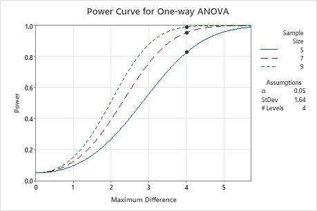
In this graph, each sample size has its own curve. The power curve for a sample size of 5 in each group shows that the test has a power of approximately 0.8 for a maximum difference of 4. The power curve for a sample size of 7 shows that the test has a power of approximately 0.95 for a maximum difference of 4. The power curve for a sample size of 9 shows that the test has a power that approaches 1.0 for a maximum difference of 4. For each sample size curve, as the maximum difference increases, the power also increases.