Alpha level
The significance level (denoted by alpha or α) is the maximum acceptable level of risk for rejecting the null hypothesis when the null hypothesis is true (type 1 error). For example, if you perform a one-way ANOVA using the default hypotheses, an α of 0.05 indicates a 5% risk of concluding that a difference exists when a difference does not actually exist.
Interpretation
Use the significance level to minimize the power value of the test when the null hypothesis (H0) is true. Higher values for the significance level give the test more power, but also increase the chance of making a type I error, which is rejecting the null hypothesis when it is true.
Assumed standard deviation
The standard deviation is the most common measure of dispersion, or how much the data vary relative to the mean. Variation that is random or natural to a process is often referred to as noise.
Interpretation
The assumed standard deviation is a planning estimate of the population standard deviation that you enter for the power analysis. Minitab uses the assumed standard deviation to calculate the power of the test. Higher values of the standard deviation indicate that there is more variation in the data, which decreases the statistical power of a test.Maximum difference
The maximum difference is the difference between the smallest group mean and the largest group mean.
Interpretation
If you enter the sample size and the power, Minitab calculates the maximum difference. Generally, larger sample sizes enable you to detect a smaller maximum difference at a specified power.
- With 5 observations in each group, the power of the test is 0.9 when the difference is approximately 4.4.
- With 7 observations in each group, the power of the test is 0.9 when the difference is approximately 3.6.
- With 9 observations in each group, the power of the test is 0.9 when the difference is approximately 3.1.
To more fully investigate the relationship between the sample size and the difference that you can detect, use the power curve.
Results
| Sample Size | Power | Maximum Difference |
|---|---|---|
| 5 | 0.9 | 4.42404 |
| 7 | 0.9 | 3.58435 |
| 9 | 0.9 | 3.09574 |
Power
The power of a one-way ANOVA is the probability that the test will determine that the maximum difference between group means is statistically significant, when that difference truly exists.
Interpretation
If you entered the maximum difference and sample size, Minitab calculates the power of the test. A power value of 0.9 is usually considered adequate. A value of 0.9 indicates that you have a 90% chance of detecting a difference between at least two of the means when that difference actually exists in the populations. If a test has low power, you might fail to detect a difference and mistakenly conclude that none exists. Usually, when the sample size is smaller or the difference is smaller, the test has less power to detect a difference.
For example, in the following results, a sample size of 4 provides a power of approximately 0.9 for a maximum difference of 6, but only 0.69 for a maximum difference of 4. At each maximum difference value, increasing the sample size increases the power of the test.
Results
| Maximum Difference | Sample Size | Power |
|---|---|---|
| 2 | 4 | 0.206970 |
| 2 | 6 | 0.332203 |
| 2 | 8 | 0.454971 |
| 4 | 4 | 0.688630 |
| 4 | 6 | 0.909626 |
| 4 | 8 | 0.978713 |
| 6 | 4 | 0.968086 |
| 6 | 6 | 0.999226 |
| 6 | 8 | 0.999988 |
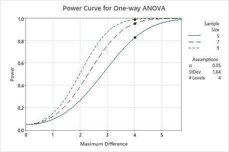
Power curve
The power curve plots the power of the test versus the maximum difference between the smallest mean and the largest mean.
Interpretation
Use the power curve to assess the appropriate sample size or power for your test.
The power curve represents every combination of power and the maximum difference for each sample size when the significant level and the standard deviation are held constant. Each symbol on the power curve represents a calculated value based on the values that you enter for two properties. For example, if you enter a sample size and a power value, Minitab calculates the corresponding maximum difference and displays the value on the graph.
Examine the values on the curve to determine the maximum difference that the test can detect at a specific power and sample size. A power value of 0.9 is usually considered adequate. However, some practitioners consider a power value of 0.8 to be adequate. If a one-way ANOVA has low power, you might fail to detect a difference between the smallest mean and the largest mean when one truly exists.
If you increase the sample size, the power of the test also increases. You want enough observations in your sample to achieve adequate power. But you don't want a sample size so large that you waste time and money on unnecessary sampling or detect unimportant differences to be statistically significant.
In this graph, each sample size has its own curve. The power curve for a sample size of 5 (in each group) shows that the test has a power of approximately 0.8 for a maximum difference of 4. The power curve for a sample size of 7 shows that the test has a power of approximately 0.95 for a maximum difference of 4. The power curve for a sample size of 9 shows that the test has a power approaching 1.0 for a maximum difference of 4. For each sample size curve, as the maximum difference increases, the power also increases.
Sample size
The sample size is the total number of observations in the sample.
Interpretation
If you enter the power and the maximum difference, Minitab calculates how large your sample must be. Sample size refers to the number of observations in each group. Because sample sizes are whole numbers, the actual power of the test might be slightly greater than the power value that you specify.
If you increase the sample size, the power of the test also increases. You want enough observations in your sample to achieve adequate power. But you don't want a sample size so large that you waste time and money on unnecessary sampling or detect unimportant differences to be statistically significant.
For example, the following results show that, for a maximum difference of 4, a larger sample size yields higher power. A sample size of 5 in each group produces an actual power of approximately 0.83, and a sample size of 6 produces an actual power of approximately 0.91.
Results
| Maximum Difference | Sample Size | Target Power | Actual Power |
|---|---|---|---|
| 4 | 5 | 0.8 | 0.826860 |
| 4 | 6 | 0.9 | 0.909626 |