Methods and formulas for Fitted Line Plot

Select the method or formula of your choice.

In This Topic

Polynomial regression models
Coefficient (Coef)
S
R-sq
R-sq (adj)
Degrees of freedom (DF)
Adj SS
Adj MS – Error
Adj MS – Regression
Adj MS – Total
F-value
P-value – Analysis of variance table
Residual (Resid)

Polynomial regression models

Formula

You can fit the following linear, quadratic, or cubic regression models:

Model type	Order	Statistical model
linear	first	Y = β₀+ β₁x + e
quadratic	second	Y = β₀+ β₁x + β₂x²+ e
cubic	third	Y = β₀+ β₁x + β₂x²+ β₃x³+ e

Another way of modeling curvature is to generate additional models by using the log10 of x and/or y for linear, quadratic, and cubic models. In addition, taking the log10 of Y may be used to reduce right-skewness or nonconstant variance of residuals.

When Minitab fits the quadratic or cubic models, Minitab standardizes the predictors before it estimates the coefficients. The standardization reduces the multicollinearity among the predictors. The reduction ensures that the multicollinearity is so low that Minitab is unlikely to exclude any predictors from the model. The output shows the unstandardized coefficients in the original units of the predictors."

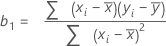
Coefficient (Coef)

The formula for the coefficient or slope in simple linear regression is:

The formula for the intercept (b₀) is:

In matrix terms, the formula that calculates the vector of coefficients in multiple regression is:

b = (X'X)^-1X'y

Notation

Term	Description
y_i	i^th observed response value
	mean response
x_i	i^th predictor value
	mean predictor
X	design matrix
y	response matrix

S

Notation

Term	Description
MSE	mean square error

R-sq

Another presentation of the formula is:

R² can also be calculated as the squared correlation of y and .

Notation

Term	Description
SS	Sum of Squares
y	response variable
	fitted response variable

R-sq (adj)

Notation

Term	Description
MS	Mean Square
SS	Sum of Squares
DF	Degrees of Freedom

Degrees of freedom (DF)

The degrees of freedom for each component of the model are:

Sources of variation	DF
Regression	p
Error	n – p – 1
Total	n – 1

If your data meet certain criteria and the model includes at least one continuous predictor or more than one categorical predictor, then Minitab uses some degrees of freedom for the lack-of-fit test. The criteria are as follows:

The data contain multiple observations with the same predictor values.
The data contain the correct points to estimate additional terms that are not in the model.

Notation

Term	Description
n	number of observations
p	number of coefficients in the model, not counting the constant

Adj SS

The sum of the squared distances. SS Regression is the portion of the variation explained by the model. SS Error is the portion not explained by the model and is attributed to error. SS Total is the total variation in the data.

Formula

SS Regression:

SS Error:

SS Total:

Notation

Term	Description
y_i	i ^th observed response value
	i ^th fitted response
	mean response

Adj MS – Error

The Mean Square of the error (also abbreviated as MS Error or MSE, and denoted as s²) is the variance around the fitted regression line. The formula is:

Notation

Term	Description
y_i	i^th observed response value
	i^th fitted response
n	number of observations
p	number of coefficients in the model, not counting the constant

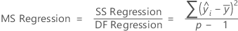
Adj MS – Regression

The formula for the Mean Square (MS) of the regression is:

Notation

Term	Description
	mean response
	i^th fitted response
p	number of terms in the model

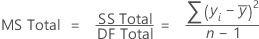
Adj MS – Total

The formula for the total Mean Square (MS) is:

Notation

Term	Description
	mean response
y_i	i^th observed response value
n	number of observations

F-value

The formulas for the F-statistics are as follows:

F(Regression)
F(Term)
F(Lack-of-fit)

Notation

Term	Description
MS Regression	A measure of the variation in the response that the current model explains.
MS Error	A measure of the variation that the model does not explain.
MS Term	A measure of the amount of variation that a term explains after accounting for the other terms in the model.
MS Lack-of-fit	A measure of variation in the response that could be modeled by adding more terms to the model.
MS Pure error	A measure of the variation in replicated response data.

P-value – Analysis of variance table

The p-value is a probability that is calculated from an F-distribution with the degrees of freedom (DF) as follows:

Numerator DF: sum of the degrees of freedom for the term or the terms in the test
Denominator DF: degrees of freedom for error

Formula

1 − P(F ≤ f_j)

Notation

Term	Description
P(F ≤ f)	cumulative distribution function for the F-distribution
f	f-statistic for the test

Residual (Resid)

Notation

Term	Description
e_i	i ^th residual
	i ^th observed response value
	i ^th fitted response