What is orthogonality?
Two vectors are orthogonal if the sum of the products of their corresponding elements is 0. For example, consider the following vectors a and b:
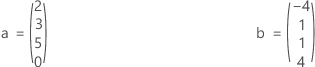
You can multiply the corresponding elements of the vectors to show the following result:
a*b = 2(–4) + 3(1) + 5(1) + 0(4) = –8 + 3 + 5 + 0 = 0
This shows that the two vectors are orthogonal.
The concept of orthogonality is important in Design of Experiments because it says something about independence. Experimental analysis of an orthogonal design is usually straightforward because you can estimate each main effect and interaction independently. If your design is not orthogonal, either by plan or by accidental loss of data, your interpretation might not be as straightforward.
| A | B | C |
|---|---|---|
| 1 | –1 | –1 |
| 1 | –1 | 1 |
| –1 | –1 | 1 |
| –1 | 1 | –1 |
| –1 | 1 | 1 |
| –1 | –1 | –1 |
| 1 | 1 | 1 |
| 1 | 1 | –1 |
- A*B = 1(–1) +1(–1) – 1(–1) – 1(1) – 1(1) – 1(–1) + 1(1) + 1(1) = –4 + 4 = 0
- A*C = 1(–1) +1(1) – 1(1) – 1(–1) – 1(1) – 1(–1) + 1(1) + 1(–1) = –4 + 4 = 0
- B*C = –1(–1) – 1(1) – 1(1) + 1(–1) + 1(1) – 1(–1) + 1(1) + 1(–1) = –4 + 4 = 0
So in a sense, factor A is estimated independently from B and C and vice versa.
The estimates for the effects and coefficients will remained unchanged when you remove interactions from the model. The other output will change as the experimental error (MSE) is adjusted accordingly with more degrees of freedom.
In conclusion, a designed experiment is orthogonal if the effects of any factor balance out (sum to zero) across the effects of the other factors. Orthogonality guarantees that the effect of one factor or interaction can be estimated separately from the effect of any other factor or interaction in the model.
Determine whether a design is orthogonal
Note
When analyzing factorial designs, if the design is displayed in uncoded units in the worksheet, first choose , select Coded units, and click OK.
-
Choose
or
and complete the dialog box as usual.
Note
You can also do this for Response Surface, Taguchi, and Mixture designs. To store a design matrix in Taguchi, you must be fitting a linear model.
- Click Storage.
- Select Design matrix. Click OK in each dialog box.
- Sum the degrees of freedom for all terms in the model, except Error. The degrees of freedom are in the DF column of the ANOVA table.
- Choose .
- In Copy from matrix, enter XMAT1.
- Under Store Copied Data, in In current worksheet, in columns:, enter a range of empty columns large enough to include a column for each degree of freedom in the model plus one for the intercept. (For example, if you have 7 degrees of freedom in your model, you will need 8 columns total and could enter C11-C18.) Click OK.
- Choose .
- In Variables, enter the range of columns from step 7.
- Click OK.
-
In the matrix, look for any nonzero terms. A positive or negative
value indicates that the two columns and their associated terms are not
orthogonal.
Note
When analyzing a factorial design, the design matrix will store the terms in uncoded units if the worksheet is in uncoded units. will perform the analysis in coded units. When analyzing a response surface design, the design matrix will store the terms in coded or uncoded units depending on the units in which you choose to analyze the data.