In This Topic
Multiple comparisons test
Multiple comparison intervals for k > 2 samples
Let  be k > 2 independent samples, each sample being independent and identically distributed with mean
  and variance
  . And, suppose that the samples originate from populations that have a common kurtosis.
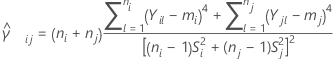
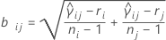
And let  be a pooled kurtosis estimator for the pair of samples ( i, j) given as:
Let  be the upper a point of the range of k variables that are independent and identically distributed on a standard normal random distribution. That is,
  satisfies the following:

where Z1, ..., Zk are independent and identically distributed standard normal random variables. Barnard (1978) provides a simple numerical algorithm based on a 16-point Gaussian quadrature for calculating the distribution function of the normal range.
The multiple comparison procedure rejects the null hypothesis of equality of variances (also called homogeneity of variances) if, and only if, at least one pair of the following intervals do not overlap:

where
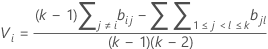
where ri = (ni - 3) / ni.
We refer to the above intervals as multiple comparison intervals or MC intervals. The MC intervals for each sample are not to be interpreted as confidence intervals for the standard deviations of the parent populations. Hochberg et al. (1982) refer to similar intervals for comparing means as "uncertainty intervals". The MC intervals given here are useful only for comparing the standard deviations or variances for multi-sample designs. When the overall multiple comparison test is significant, the standard deviations that correspond to the non-overlapping intervals are statistically different. (For the detailed derivation of these intervals, go to the white paper on Multiple comparison methods.)
Multiple comparison intervals for k = 2 samples
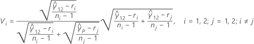
When there are only two samples, the multiple comparison intervals are given by:

where zα / 2 is the upper α / 2 percentile point of the standard normal distribution, ci = ni / ni - zα / 2, and Vi is given by the following formula:
P-value for the test
If there are 2 samples in the design, then Minitab calculates the p-value for the multiple comparisons test using Bonett's method for a 2 variances test and a hypothesized ratio, Ρo, of 1.
If there are k > 2 samples in the design, then let Pi j be the p-value of the test for any pair (i, j ) of samples. The p-value for the multiple comparisons procedure as an overall test of equality of variances is given by the following:

For more information, including simulations and detailed algorithms for calculating Pi j , go to Bonett's Method, which is a white paper that has simulations and other information about Bonett's Method.
Notation
| Term | Description |
|---|---|
| ni | the number of observations in sample i |
| Y i l | the lth observation in sample i |
| mi | the trimmed mean for sample i with trim proportions of  |
| k | the number of samples |
| Si | the standard deviation of sample i |
| α | the significance level for the test = 1 - (the confidence level / 100) |
| Ci |  |
| Zα / 2 | the upper α / 2 percentile point of the standard normal distribution |
| ri |  |
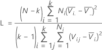
Levene's test statistic
Minitab displays a test statistic and a p-value for Levene's test. The null hypothesis is that the variances are equal, and the alternative hypothesis is that the variances are not equal. Use Levene's test when the data come from continuous, but not necessarily normal, distributions.
The calculation method for Levene's test is a modification of Levene's procedure (Levene, 1960) that was developed by Brown and Forsythe (1974). This method considers the distances of the observations from their sample median rather than their sample mean. Using the sample median rather than from the sample mean makes the test more robust for smaller samples and makes the procedure asymptotically distribution-free. If the p-value is smaller than your α-level, reject the null hypothesis that the variances are equal.
Formula
- H. Levene (1960). Contributions to Probability and Statistics. Stanford University Press, CA.
- M. B. Brown and A. B. Forsythe (1974). "Robust tests for the equality of variance," Journal of the American Statistical Association, 69, 364-367.
Notation
| Term | Description |
|---|---|
| Vij |  |
| i | 1, ..., k |
| j | 1, ..., ni |
 | median |
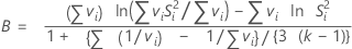
Bartlett's test statistic
Minitab displays a test statistic and a p-value for Bartlett's test. When there are only two levels, Minitab performs an F-test instead of Bartlett's test. For these tests, the null hypothesis is that the variances are equal, and the alternative hypothesis is that the variances are not equal. Use Bartlett's test when the data are from normal distributions; Bartlett's test is not robust to departures from normality.
Bartlett's test statistic calculates the weighted arithmetic average and weighted geometric average of each sample variance based on the degrees of freedom. The greater the difference in the averages, the more likely the variances of the samples are not equal. B follows a χ2 distribution with k – 1 degrees of freedom. If the p-value is smaller than your α-level, reject the null hypothesis that the variances are equal.
Formula
Notation
| Term | Description |
|---|---|
| si2 | 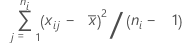 |
| k | number of samples |
| vi | ni - 1 |
| ni | number of observations at the ith factor level |
F-test statistic
When there are only two levels, Minitab performs an F-test instead of Bartlett's test. The null hypothesis is that the variances are equal, and the alternative hypothesis is that the variances are not equal. Use the F-statistic when the data are from normal distributions.
If the p-value is less than the α-level, reject the null hypothesis that the variances are equal.
Formula

Formula for p-value
- For a one-sided test with an alternative hypothesis of less than, the p-value equals the probability of obtaining an F-statistic that is equal to or less than the observed value from an F-distribution with degrees of freedom DF1 and DF2.
- For a two-sided test where the ratio is less than 1, the p-value equals two times the area under the F-curve less than the observed value from an F-distribution with degrees of freedom DF1 and DF2.
- For a two-sided test where the ratio is greater than 1, the p-value equals two times the area under the F-curve greater than the observed value from an F-distribution with degrees of freedom DF1 and DF2.
- For a one-sided test with an alternative hypothesis of greater than, the p-value equals the probability of obtaining an F-statistic that is equal to or greater than the observed value from an F-distribution with degrees of freedom DF1 and DF2.
Notation
| Term | Description |
|---|---|
| S12 | variance of sample 1 |
| S22 | variance of sample 2 |
| n1 - 1 | degrees of freedom for numerator |
| n2 - 1 | degrees of freedom for denominator |
Standard deviation (StDev)
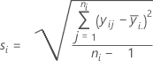
Notation
| Term | Description |
|---|---|
| yij | observations at the ith factor level |
 | mean of observations at the ith factor level |
| ni | number of observations at the ith factor level |
Bonferroni confidence intervals
Minitab calculates confidence intervals for the standard deviations using the Bonferroni method. A confidence interval is a range of values that is likely to include some population parameter, in this case, contain the standard deviation.
Standard confidence intervals are calculated using a confidence level 1 – α / 2. the Bonferroni method uses the confidence level 1 – α / 2p for each individual confidence interval, where p is the number of factor and level combinations. The method ensures that the set of confidence intervals has a confidence level of at least 1 – α. The Bonferroni method provides more conservative (wider) confidence intervals, which reduces the probability of a type 1 error.