In This Topic
Sum of squares (SS)
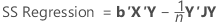
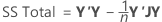
In matrix terms, these are the formulas for the different sums of squares:

Minitab breaks down the SS Regression or SS Treatments component into the amount of variation explained by each term using both the sequential sum of squares and adjusted sum of squares.
Notation
| Term | Description |
|---|---|
| b | vector of coefficients |
| X | design matrix |
| Y | vector of response values |
| n | number of observations |
| J | n by n matrix of 1s |
Sequential sum of squares
Minitab breaks down the SS Regression or Treatments component of variance into sequential sums of squares for each factor. The sequential sums of squares depend on the order the factors or predictors are entered into the model. The sequential sum of squares is the unique portion of SS Regression explained by a factor, given any previously entered factors.
For example, if you have a model with three factors or predictors, X1, X2, and X3, the sequential sum of squares for X2 shows how much of the remaining variation X2 explains, given that X1 is already in the model. To obtain a different sequence of factors, repeat the analysis and enter the factors in a different order.
Adjusted sum of squares
The adjusted sums of squares does not depend on the order that the terms enter the model. The adjusted sum of squares is the amount of variation explained by a term, given all other terms in the model, regardless of the order that the terms enter the model.
For example, if you have a model with three factors, X1, X2, and X3, the adjusted sum of squares for X2 shows how much of the remaining variation the term for X2 explains, given that the terms for X1 and X3 are also in the model.
The calculations for the adjusted sums of squares for three factors are:
- SSR(X3 | X1, X2) = SSE (X1, X2) - SSE (X1, X2, X3) or
- SSR(X3 | X1, X2) = SSR (X1, X2, X3) - SSR (X1, X2)
where SSR(X3 | X1, X2) is the adjusted sum of squares for X3, given that X1 and X2 are in the model.
- SSR(X2, X3 | X1) = SSE (X1) - SSE (X1, X2, X3) or
- SSR(X2, X3 | X1) = SSR (X1, X2, X3) - SSR (X1)
where SSR(X2, X3 | X1) is the adjusted sum of squares for X2 and X3, given that X1 is in the model.
You can extend these formulas if you have more than 3 factors in your model1.
- J. Neter, W. Wasserman and M.H. Kutner (1985). Applied Linear Statistical Models, Second Edition. Irwin, Inc.
Degrees of freedom (DF)
The degrees of freedom for each component of the model are:
| Sources of variation | DF |
|---|---|
| Factor | ki – 1 |
| Covariates and interactions between covariates | 1 |
| Interactions that involve factors |  |
| Regression | p |
| Error | n – p – 1 |
| Total | n – 1 |
- The data contain multiple observations with the same predictor values.
- The data contain the correct points to estimate additional terms that are not in the model.
Notation
| Term | Description |
|---|---|
| ki | number of levels in the ith factor |
| m | number of factors |
| n | number of observations |
| p | number of coefficients in the model, not counting the constant |
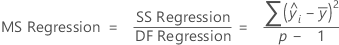
Adj MS – Regression
The formula for the Mean Square (MS) of the regression is:
Notation
| Term | Description |
|---|---|
 | mean response |
 | ith fitted response |
| p | number of terms in the model |
Adj MS – Error
The Mean Square of the error (also abbreviated as MS Error or MSE, and denoted as s2) is the variance around the fitted regression line. The formula is:

Notation
| Term | Description |
|---|---|
| yi | ith observed response value |
 | ith fitted response |
| n | number of observations |
| p | number of coefficients in the model, not counting the constant |
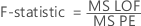
F
If all the factors in the model are fixed, then the calculation of the F-statistic depends on what the hypothesis test is about, as follows:
- F(Term)
-

- F(Lack-of-fit)
-

If there are random factors in the model, F is constructed using the expected mean square information for each term. For more information, see Neter et al.1.
Notation
| Term | Description |
|---|---|
| Adj MS Term | A measure of the amount of variation that a term explains after accounting for the other terms in the model. |
| MS Error | A measure of the variation that the model does not explain. |
| MS Lack-of-fit | A measure of variation in the response that could be modeled by adding more terms to the model. |
| MS Pure error | A measure of the variation in replicated response data. |
- J. Neter, W. Wasserman and M.H. Kutner (1985). Applied Linear Statistical Models, Second Edition. Irwin, Inc.
P-value – Analysis of variance table
The p-value is a probability that is calculated from an F-distribution with the degrees of freedom (DF) as follows:
- Numerator DF
- sum of the degrees of freedom for the term or the terms in the test
- Denominator DF
- degrees of freedom for error
Formula
1 − P(F ≤ fj)
Notation
| Term | Description |
|---|---|
| P(F ≤ f) | cumulative distribution function for the F-distribution |
| f | f-statistic for the test |
Pure error lack-of-fit test
- The sum of squared deviations of the response from the mean within each set of replicates and adds them together to create the pure error sum of squares (SS PE).
- The pure error mean square


where n = number of observations and m = number of distinct x-level combinations
- The lack-of-fit sum of squares

- The lack-of-fit mean square

- The test statistics
Large F-values and small p-values suggest that the model is inadequate.
P-value – Lack-of-fit test
- Numerator DF
- degrees of freedom for lack-of-fit
- Denominator DF
- degrees of freedom for pure error
Formula
1 − P(F ≤ fj)
Notation
| Term | Description |
|---|---|
| P(F ≤ fj) | cumulative distribution function for the F-distribution |
| fj | f-statistic for the test |