Report 7: Product Performance
Six Sigma Product Report
- Component
- Optional column to provide names for components. If you don't specify names, Minitab assign numbers as IDs.
- Obs Defs
- Number of defects observed.
- Obs Units
- Number of units of each component observed.
- Opps per Unit
-
Number of opportunities (for defect) per unit.
For more information, go to What is opportunities per unit?.
- Cmplx
-
Complexity counts for each component. You can adjust the observed units and observed defects by setting proportions for each component. For example, to make a larger assembly, you need 1 unit of component 1, 6 units of component 2, 5 units of component 3, and so on.
The complexity column is not required, but using complexity values reduces the effects of disproportionate sampling. If there are no proportions, enter a column of all 1s.
For more information, go to What is complexity?.
- Adj Defs
- Observed defects are adjusted (or weighted) based on the complexity information. When no complexity units are given, adjusted defects are the same as observed defects.
- Adj Units
- Observed units are adjusted (or weighted) based on the complexity information. When no complexity units are given, adjusted units are the same as observed units. All components that have the same complexity have the same adjusted units. In the example, components 7 and 12 both have complexity of 3 and adjusted units of 234.
- Adj Total Opps
- This column is calculated by multiplying Adj Units and Opps per Unit. If the unit counts were not adjusted, the total opportunities would be skewed in favor of components with larger numbers of observed units, which would affect the calculations of performance statistics. Again, using complexity values reduces the effects of disproportionate sampling.
- DPU
- Defects per unit, calculated by dividing the number of defects by the number of units.
- DPMO
-
Defects per million opportunities, calculated by dividing Adj Units by Adj Tot Opps, then multiplying by 1 million.
If the unit counts were not adjusted, the total opportunities would be skewed in favor of components with larger numbers of observed units.
- Z.Shift
-
Values to represent the assumed long-term sigma shift. If one is not specified, Minitab uses the default values of 1.5.
For more information, go to Z.bench as an estimate of sigma capability.
- Z.ST
- Z scores calculated from DPMO and Z.Shift.
- YTP
-
Throughput yield for each component. This is the probability that none of the opportunities in the component result in a defect.
For more information, go to What are throughput yield (YTP) and rolled throughput yield (YRT)?.
- YRT
-
Rolled throughput yield for each component. The probability of having one good unit of component 2 is the YTP, 0.996698. To make a larger assembly, you need 6 units of component 2. The probability of having 6 good units of component 2 is the YRT, (0.996698)6 = 0.980350.
For more information, go to What are throughput yield (YTP) and rolled throughput yield (YRT)?.
Report 8A: Product Benchmarks (DPMO versus Z.Bench)
The Product Benchmarks (DPMO versus Z.Bench) report displays a graphical view of the benchmark statistics for the collection of components that are in the product report.
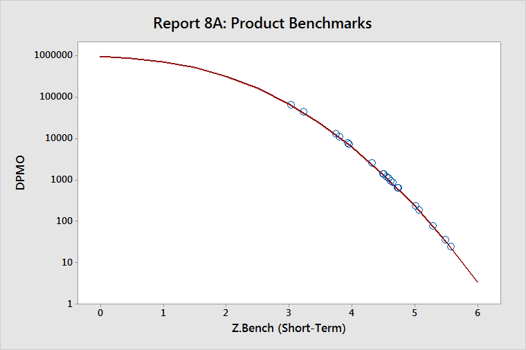
DPMO is a measure of long-term performance. Z.Bench ST is a measure of short-term performance.
The locations of the clusters of points represent where the capabilities of your processes tend to be concentrated. In the example above, there is a cluster just below 4 on the Z.ST scale, and another near 4.5. Thus, many of the processes used here run from just under 4 to just over 4 sigma. This is quite typical.
Report 8B: Product Benchmarks (Z.Shift versus Z.Bench)
The Product Benchmarks (Z.Shift versus Z.Bench) report displays another view of the benchmark statistics for the collection of components that are in the product report.
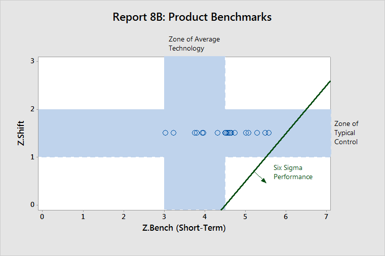
This graph compares the controllability of each component (Z.Shift) and the capability of each component (Z.ST). Typically, Z.Shift values fall within the horizontal band (Zone of Typical Control) and Z.ST values fall within the vertical band (Zone of Average Technology).
Six Sigma Performance is achieved at high levels of Z.Bench and low levels of Z.Shift.
Z.Shift
- Low Z.Shift values correspond to characteristics that are very well controlled.
- High Z.Shift values correspond to characteristics that are poorly controlled.
Z.Bench ST
- High Z.Bench values correspond to characteristics that represent technological superiority.
- Low Z.Bench values correspond to characteristics that represent technological inferiority.
In the example above, all components had a Z.shift of 1.5 sigma, which is the default when actual Z.Shift values are unknown. About half of the components have Z.Bench values in the Zone of Average Technology. The other half of the components have values to the right, which indicates better than average capability.
Report 8C: Product Benchmarks (Capability, Complexity, Control)
Without complexity information
- YTP: A reverse Pareto diagram of throughput yields (YTP)
- Opps per Unit: Opportunities per unit for the components, ordered by YTP values
- Z.ST: Z.ST values for the components, ordered by YTP values
- Z.Shift: Z.shift values for the components, ordered by YTP values
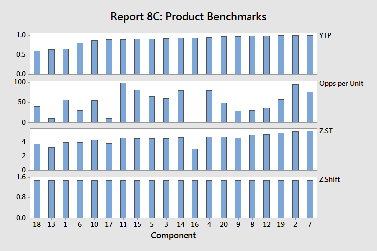
In the YTP graph, identify the components that have the worst quality, then look at the lower charts to determine whether the problem is a result of high complexity (opportunity count), low capability (Z.ST), or poor control (Z.Shift).
In the example above, component 18 has the worst quality, moderate opportunity count, and below average capability. Improving capability will have the largest impact on improving quality.
With complexity information
- YRT: A reverse Pareto diagram of rolled throughput yields (YRT)
- Total Opps per Unit: Opportunities per unit for the components, ordered by YRT values
- Z.ST: Z.ST values for the components, ordered by YRT values
- Z.Shift: Z.shift values for the components, ordered by YRT values
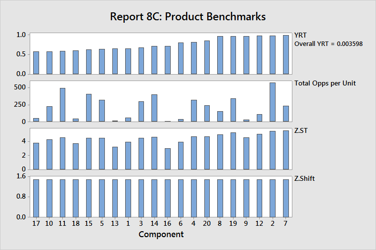
Remember, the overall YRT represents the probability that a single unit of the entire collection of components can be produced without any defects. The components that have the lowest component-level YRT values contribute the most to the overall YRT. Thus, improving those components is critical for improving overall YRT.
In the example above, component 17 has the lowest YRT, a low opportunity count, and low capability. Raising the average Z.ST for component 17 will have the largest effect on improving its quality and, thereby, improving the overall product quality.
Component 11 (the third worst component) has a high opportunity count and good capability. Reducing the opportunity count will have the largest effect on improving the quality of component 11, because the capability is already quite good.