In This Topic
Bias
The bias is a measure of a measurement system's accuracy. Bias is calculated as the difference between the known standard value of a reference part and the observed average measurement.
Interpretation
- A positive bias indicates that the gage measures high.
- A negative bias indicates that the gage measures low.
For a gage that measures accurately, the %bias will be small. To determine whether the bias is statistically significant, use the p-value.
Repeatability and pre-adjusted repeatability
Repeatability is the amount of variation in the measurement system that is from the gage. An attribute gage study regresses the probabilities of acceptance on the reference values to obtain repeatability.
Pre-adjusted repeatability is the repeatability that is calculated before adjusting for over-estimation. Minitab divides estimates of repeatability by the adjustment factor 1.08 to calculate the adjusted repeatability. The adjustment factor of 1.08 is given by the Automotive Industry Action Group (AIAG)1.
Interpretation
A low repeatability value indicates that the gage measures consistently. A high repeatability value indicates random variation, or problems such as an inadequate selection of parts or a poor gage.
Minitab uses the adjusted repeatability value in the calculation to test the null hypothesis of bias = 0.
Normal probability plot
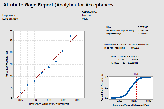
The normal probability plot shows the percent of acceptances for each reference value. Because no actual measurements from the gage are available to estimate bias and repeatability, Minitab calculates bias and repeatability by fitting the normal distribution curve using the calculated probabilities of acceptance and the known reference values for all parts.
If the measurement errors follow a normal distribution, the calculated probabilities fall along a straight line. A regression line is fit to the probabilities.
Interpretation
Fitted line
The probability of acceptance for each part is calculated and plotted on a normal probability plot. On a normal probability plot, the y-value of a plotted point = Φ–1(Probability of Acceptance), where Φ–1 is the inverse of the standard normal cumulative distribution function.
A fitted regression line is drawn through the plotted points.
Interpretation
If the fitted line is a good fit for the plotted points, Minitab uses the intercept and slope values to calculate the bias and repeatability values.
This graph shows that the fitted line fits the data well.
R-sq for fitted line
The R-sq (R2) value for the fitted regression line indicates the percentage of the variation in the probability of acceptance responses that is explained by the regression model.
Interpretation
R2 ranges from 0 to 100%. Usually, the higher the R2 value, the better the model fits your data. R2 values that are greater than 90% usually indicate a very good fit of the data.
For this example, R-sq is 0.969376. The fitted line fits the data very well, and the model accounts for almost 97% of the variance.
T
T is the t-statistic for the alternative hypothesis that bias ≠ 0.
The t-test compares this observed t-statistic to a critical value on the t-distribution with (n-1) degrees of freedom to determine whether the bias in the measurement system is statistically significant.
DF
The degrees of freedom (DF) value is used to determine the p-value. For the AIAG method, DF = the number of trials –1. For the regression method, DF is the number of points used to create the fitted line –2.
P-value
To determine whether bias in the measurement system is statistically significant, compare the p-value to the significance level. Usually, a significance level (denoted as α or alpha) of 0.05 works well. A significance level of 0.05 indicates a 5% risk of concluding that bias exists when there is no significant bias.
Interpretation
A smaller p-value provides stronger evidence against the null hypothesis. If the p-value is less than the α-value, you can reject the null hypothesis that the bias in the measurement system is equal to 0.
Gage performance curve
The gage performance curve shows the estimated probability of acceptance as a function of the reference value for the item. The vertical reference line indicates the limit(s) you entered for the analysis.
Interpretation
If you specify a lower tolerance limit, the reference values and probabilities of acceptance show an increasing trend. If you specify an upper tolerance limit, as the reference values increase, the probabilities of acceptance decrease.
If a gage has an upper and lower limit and you can assume linearity and uniformity of error, you can show both upper and lower tolerance limits on the gage performance curve. The curve appears as a mirror image.
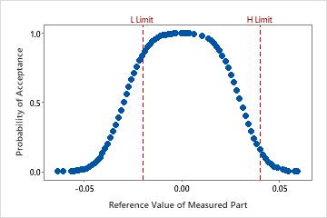
For this data, the probability of accepting an item at the lower tolerance limit (L Limit) of −0.020 is high. The probability of acceptance increases as the reference values increase until the reference value of 0.01. Then the probability of acceptance declines. The probability of acceptance at the upper tolerance limit (H Limit) is approximately 0.15 probability.