In This Topic
α (alpha)
The significance level (denoted as α or alpha) is the maximum acceptable level of risk for rejecting the null hypothesis when the null hypothesis is true (type I error). Alpha is also interpreted as the power of the test when the null hypothesis (H0) is true. Usually, you choose the significance level before you analyze the data. The default significance level is 0.05.
Interpretation
Use the significance level to minimize the power value of the test when the null hypothesis (H0) is true. Higher values for the significance level give the test more power, but also increase the chance of making a type I error, which is rejecting the null hypothesis when it is true.
Ratio
This value represents the ratio between the comparison standard deviation or variance and the hypothesized value.
Interpretation
Minitab calculates the smallest ratio that you will be able to detect based on your specified power and sample size. Larger sample sizes allow you to detect smaller ratios. You want to be able to detect the smallest ratio that has practical consequences for your application.
To more fully investigate the relationship between the sample size and the ratio at a given power, use the power curve.
Sample Size
The sample size is the total number of observations in the sample.
Interpretation
Use the sample size to estimate how many observations you need to obtain a certain power value for the hypothesis test at a specific difference.
Minitab calculates how large your sample must be for a test with your specified power to detect the specified ratio. Because sample sizes are whole numbers, the actual power of the test might be slightly greater than the power value that you specify.
If you increase the sample size, the power of the test also increases. You want enough observations in your sample to achieve adequate power. But you don't want a sample size so large that you waste time and money on unnecessary sampling or detect unimportant differences to be statistically significant.
To more fully investigate the relationship between the sample size and the difference at a given power, use the power curve.
Power
The power of a hypothesis test is the probability that the test correctly rejects the null hypothesis. The power of a hypothesis test is affected by the sample size, the difference, the variability of the data, and the significance level of the test.
For more information, go to What is power?.
Interpretation
Minitab calculates the power of the test based on the specified ratio and sample size. A power value of 0.9 is usually considered adequate. A value of 0.9 indicates you have a 90% chance of detecting a difference between the population comparison standard deviation or variance and the hypothesized standard deviation or variance when a difference actually exists. If a test has low power, you might fail to detect a difference and mistakenly conclude that none exists. Usually, when the sample size is smaller or the ratio is closer to 1, the test has less power to detect a difference.
If you enter a ratio and a power value for the test, then Minitab calculates how large your sample must be. Minitab also calculates the actual power of the test for that sample size. Because sample sizes are whole numbers, the actual power of the test might be slightly greater than the power value that you specify.
Note
When you perform 1 Variance in Basic Statistics, Minitab displays output for both the chi-square method and the Bonett method. However, when you perform Power and Sample Size for 1 Variance, Minitab uses only the chi-square method.
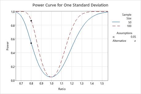
Power curve
The power curve plots the power of the test versus the ratio.
Interpretation
Use the power curve to assess the appropriate sample size or power for your test.
The power curve represents every combination of power and ratio for each sample size when the significance level is held constant. Each symbol on the power curve represents a calculated value based on the values that you enter. For example, if you enter a sample size and a power value, Minitab calculates the corresponding ratio and displays the calculated value on the graph.
Examine the values on the curve to determine the ratio that can be detected at a certain power value and sample size. A power value of 0.9 is usually considered adequate. However, some practitioners consider a power value of 0.8 to be adequate. If a hypothesis test has low power, you might fail to detect a ratio that is practically significant. If you increase the sample size, the power of the test also increases. You want enough observations in your sample to achieve adequate power. But you don't want a sample size so large that you waste time and money on unnecessary sampling or detect unimportant differences to be statistically significant. If you decrease the size of the ratio that you want to detect, the power also decreases.
Note
When you perform 1 Variance in Basic Statistics, Minitab displays output for both the chi-square method and the Bonett method. However, when you perform Power and Sample Size for 1 Variance, Minitab uses only the chi-square method.
In this graph, the power curve for a sample size of 50 shows that the test has a power of approximately 0.54 for a ratio of 0.8. For a sample size of 100, the power curve shows that the test has a power of approximately 0.87 for a ratio of 0.8. If a power of 0.87 is adequate for your situation, you should collect a sample size of 100. If you need to detect a ratio smaller than 0.8, you will need to collect a larger sample.