In This Topic
Mean
A commonly used measure of the center of a batch of numbers. The mean is also called the average. It is the sum of all observations divided by the number of (nonmissing) observations.
Formula

Notation
| Term | Description |
|---|---|
| xi | ith observation |
| N | number of nonmissing observations |
Standard deviation (StDev)
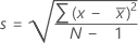
The sample standard deviation provides a measure of the spread of your data. It is equal to the square root of the sample variance.
Formula
 , then the standard deviation of the sample is:
Notation
| Term | Description |
|---|---|
| x i | i th observation |
 | mean of the observations |
| N | number of nonmissing observations |
N
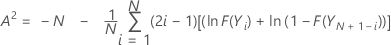
Anderson-Darling statistic (A2)
A2 measures the area between the fitted line (which is based on the chosen distribution) and the nonparametric step function (which is based on the plot points). The statistic is a squared distance that is weighted more heavily in the tails of the distribution. A small Anderson-Darling value indicates that the distribution fits the data better.
The Anderson-Darling normality test is defined as:
H0: The data follow a normal distribution
H1: The data do not follow a normal distribution
Formula
Notation
| Term | Description |
|---|---|
| F(Yi) |  , which is the cumulative distribution function of the standard normal distribution , which is the cumulative distribution function of the standard normal distribution |
| Yi | ordered data |
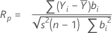
Ryan-Joiner
The Ryan-Joiner test provides a correlation coefficient, which indicates the correlation between your data and the normal scores of your data. If the correlation coefficient is near 1, your data falls close to the normal probability plot. If it is less than the appropriate critical value, you will reject the null hypothesis of normality.
Formula
Notation
| Term | Description |
|---|---|
| Yi | ordered observations |
| bi | normal scores of your ordered data |
| s2 | sample variance |
Kolmogorov-Smirnov
Formula
- H0: The data follow a normal distribution
- H1: The data do not follow a normal distribution

Notation
| Term | Description |
|---|---|
| D+ | maxi {i / n – Z (i)} |
| D– | maxi {Z (i) – (i – 1) / n)} |
| Z | F(X(i)) |
| F(x) | probability distribution function of the normal distribution |
| X(i) | ith order statistics of a random sample, 1 ≤ i ≤ n |
| n | sample size |
P-value
Another quantitative measure for reporting the result of the normality test is the p-value. A small p-value is an indication that the null hypothesis is false.
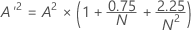
- If 13 > A'2 > 0.600 then p = exp(1.2937 - 5.709 * A'2 + 0.0186(A'2)2)
- If 0.600 > A'2 > 0.340 then p = exp(0.9177 - 4.279 * A'2 – 1.38(A'2)2)
- If 0.340 > A'2 > 0.200 then p = 1 – exp(–8.318 + 42.796 * A'2 – 59.938(A'2)2)
- If A'2 <0.200 then p = 1 – exp(–13.436 + 101.14 * A'2 – 223.73(A'2)2)
Plot points
In general, the closer the points fall to the fitted line, the better the fit. Minitab provides two goodness-of-fit measures to help assess how the distribution fits your data.
Formula
| Distribution | x coordinate | y coordinate |
|---|---|---|
| Normal | x | Φ–1 norm |
Notation
| Term | Description |
|---|---|
| Φ–1 norm | value returned for p by the inverse cdf for the standard normal distribution |
Probability plots
The input data are plotted as the x-values. Minitab calculates the probability of occurrence without assuming a distribution. The Y-scale on the graph resembles the Y scale found on normal probability paper where the probabilities plot as a straight line, as if the data are from a normal distribution.