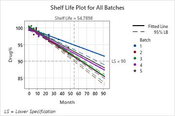
A quality engineer for a pharmaceutical company wants to determine the shelf life for pills that contain a new drug. The concentration of the drug in the pills decreases over time. The engineer wants to determine when the pills get to 90% of the intended concentration. Because this is a new drug, the company has only 5 pilot batches to use to estimate the shelf life. The engineer tests one pill from each batch at nine different times.
To estimate the shelf life, the engineer does a stability study. Because the engineer samples all of the batches, batch is a fixed factor instead of a random factor.
Choose Stat > Regression > Stability Study > Stability Study.
In Response, enter Drug%.
In Time, enter Month.
In Batch, enter Batch.
In Lower spec, enter 90.
Click Graphs.
Under Shelf life plot, in the second drop-down list, select No graphs for individual batches.
Under Residuals Plots, select Four in one.
Click OK in each dialog box.
Interpret the results
To follow the 2003 guidelines of the International Conference on Harmonisation of Technical Requirements for Registration of Pharmaceuticals for Human Use (ICH), the engineer selects a p-value of 0.25 for terms to include in the model. The p-value for the Month by Batch interaction is 0.048. Because the p-value is less than the significance level of 0.25, the engineer concludes that the slopes in the regression equations for each batch are different. Batch 3 has the steepest slope, -0.1630, which indicates that the concentration decreases the fastest in Batch 3. Batch 2 has the shortest shelf life, 54.79, so the overall shelf life is the shelf life for Batch 2.
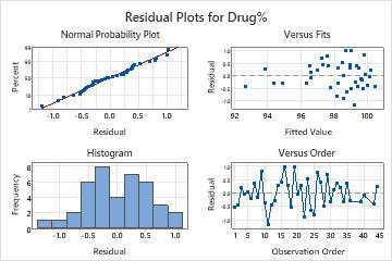
The residuals are adequately normal and randomly scattered about 0. On the residuals versus fits plot, less points are on the left side of the plot than are on the right side. This pattern occurs because the quality engineer collected more data earlier in the study when concentrations were high. This pattern is not a violation of the assumptions of the analysis.
Syntax Error
Factor Information
Factor
Type
Number of Levels
Levels
Batch
Fixed
5
1, 2, 3, 4, 5
Model Selection with α = 0.25
Source
DF
Seq SS
Seq MS
F-Value
P-Value
Month
1
122.460
122.460
345.93
0.000
Batch
4
2.587
0.647
1.83
0.150
Month*Batch
4
3.850
0.962
2.72
0.048
Error
30
10.620
0.354
Total
39
139.516
Model Summary
S
R-sq
R-sq(adj)
R-sq(pred)
0.594983
92.39%
90.10%
85.22%
Coefficients
Term
Coef
SE Coef
T-Value
P-Value
VIF
Constant
100.085
0.143
701.82
0.000
Month
-0.13633
0.00769
-17.74
0.000
1.07
Batch
1
-0.232
0.292
-0.80
0.432
3.85
2
0.068
0.292
0.23
0.818
3.85
3
0.394
0.275
1.43
0.162
3.41
4
-0.317
0.292
-1.08
0.287
3.85
5
0.088
0.275
0.32
0.752
*
Month*Batch
1
0.0454
0.0164
2.76
0.010
4.52
2
-0.0241
0.0164
-1.47
0.152
4.52
3
-0.0267
0.0136
-1.96
0.060
3.65
4
0.0014
0.0164
0.08
0.935
4.52
5
0.0040
0.0136
0.30
0.769
*
Regression Equation
Batch
1
Drug%
=
99.853 - 0.0909 Month
2
Drug%
=
100.153 - 0.1605 Month
3
Drug%
=
100.479 - 0.1630 Month
4
Drug%
=
99.769 - 0.1350 Month
5
Drug%
=
100.173 - 0.1323 Month
Fits and Diagnostics for Unusual Observations
Obs
Drug%
Fit
Resid
Std Resid
11
98.001
99.190
-1.189
-2.21
R
43
92.242
92.655
-0.413
-1.47
X
44
94.069
93.823
0.246
0.87
X
Shelf Life Estimation
Lower spec limit = 90 Shelf life = time period in which you can be 95% confident that at least 50% of response is above lower spec limit