A reliability engineer studies the failure rates of engine windings of turbine assemblies to determine the times at which the windings fail. At high temperatures, the windings might decompose too fast.
The engineer records failure times for the engine windings at 80° C and 100° C. However, some of the units must be removed from the test before they fail. Therefore, the data are right censored. The engineer uses Distribution Overview Plot (Right Censoring) to fit a lognormal distribution to the data and to visually assess the survival and failure rates over time.
- Open the sample data, EngineWindingReliability.MWX.
- Choose .
- In Variables, enter Temp80 Temp100.
- Select Parametric analysis. From Distribution, select Lognormal.
- Click Censor. Under Use censoring columns, enter Cens80 Cens100.
- In Censoring value, type 0.
- Click OK in each dialog box.
Interpret the results
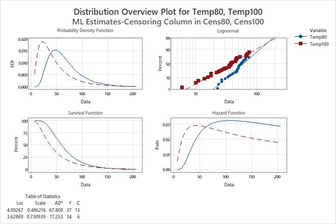
The probability plot shows that the points for the failure times fall approximately on the straight line for both variables. Therefore, the lognormal distribution is a good fit for the data for both variables.
Use the hazard function plot to compare the failure rate for different variables. For example, at 100° C, the rate of failure is initially greater than at 80° C, reaching a peak of nearly 0.03 at approximately 40 hours. At 80° C, the rate of failure increases more slowly, reaching a peak of over 0.032 at approximately 50 hours.
Use the survival function plot to compare the survival rate for different variables. For example, at times of less than approximately 150 hours, the percentage of windings that survive is considerably greater at 80° C than at 100° C. After 150 hours, the percentage of windings that survive becomes almost the same at the two temperatures.