In This Topic
S
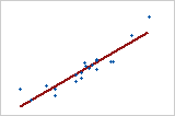
S represents the standard deviation of the distance between the data values and the fitted values. S is measured in the units of the response.
Interpretation
Use S to assess how well the model describes the response. S is measured in the units of the response variable and represents how far the data values fall from the fitted values. The lower the value of S, the better the model describes the response. However, a low S value by itself does not indicate that the model meets the model assumptions. You should check the residual plots to verify the assumptions.
For example, you work for a potato chip company that examines the factors that affect the percentage of crumbled potato chips per container. You reduce the model to the significant predictors, and S is calculated as 1.79. This result indicates that the standard deviation of the data points around the fitted values is 1.79. If you are comparing models, values that are lower than 1.79 indicate a better fit, and higher values indicate a worse fit.
R-sq
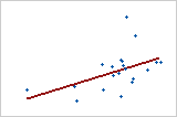
R2 is the percentage of variation in the response that is explained by the model. It is calculated as 1 minus the ratio of the error sum of squares (which is the variation that is not explained by model) to the total sum of squares (which is the total variation in the model).
Interpretation
Use R2 to determine how well the model fits your data. The higher the R2 value, the better the model fits your data. R2 is always between 0% and 100%.
-
R2 always increases when you add additional predictors to a model. For example, the best five-predictor model will always have an R2 that is at least as high as the best four-predictor model. Therefore, R2 is most useful when you compare models of the same size.
-
Small samples do not provide a precise estimate of the strength of the relationship between the response and predictors. For example, if you need R2 to be more precise, you should use a larger sample (typically, 40 or more).
-
Goodness-of-fit statistics are just one measure of how well the model fits the data. Even when a model has a desirable value, you should check the residual plots to verify that the model meets the model assumptions.
R-sq (adj)
Adjusted R2 is the percentage of the variation in the response that is explained by the model, adjusted for the number of predictors in the model relative to the number of observations. Adjusted R2 is calculated as 1 minus the ratio of the mean square error (MSE) to the mean square total (MS Total).
Interpretation
Use adjusted R2 when you want to compare models that have different numbers of predictors. R2 always increases when you add a predictor to the model, even when there is no real improvement to the model. The adjusted R2 value incorporates the number of predictors in the model to help you choose the correct model.
| Model | % Potato | Cooling rate | Cooking temp | R2 | Adjusted R2 |
|---|---|---|---|---|---|
| 1 | X | 52% | 51% | ||
| 2 | X | X | 63% | 62% | |
| 3 | X | X | X | 65% | 62% |
The first model yields an R2 of more than 50%. The second model adds cooling rate to the model. Adjusted R2 increases, which indicates that cooling rate improves the model. The third model, which adds cooking temperature, increases the R2 but not the adjusted R2. These results indicate that cooking temperature does not improve the model. Based on these results, you consider removing cooking temperature from the model.