Note
This command is available with the Predictive Analytics Module. Click here for more information about how to activate the module.
Important variables
Minitab Statistical Software offers two methods to rank the importance of the variables.
Permutation
- A = 87
- B= 9
- C = 4
Then the margin for that row is 0.87 - 0.09 = 0.78.
The average out-of-bag margin is the average margin for all of the rows of data.
To determine the importance of the variable, randomly permute the values
of a variable,
xm through the out-of-bag data. Leave the response values
and the other predictor values the same. Then, use the same steps to calculate
the average margin for the permuted data,  .
.
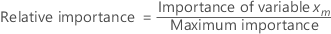
The importance for variable xm comes from the difference of the two averages:

where  is the average margin before the permutation. Minitab rounds values smaller
than 10–7 to 0.
is the average margin before the permutation. Minitab rounds values smaller
than 10–7 to 0.
Gini
Any classification tree is a collection of splits. Each split provides improvement to the tree.
The following formula gives the improvement at a single node:


where  is the number of nodes that split and
  for any node
  where the variable of interest is not the splitter.
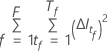
Where  is the number of trees in the forest and
  is the number of nodes that split in tree
  .
.
The calculation of node impurity is similar to the Gini method. For details on the Gini method, go to Node splitting methods in CART® Classification.

Average –loglikelihood
Out-of-bag data
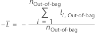
The calculation uses the out-of-bag samples from every tree in the forest. Because of the nature of out-of-bag samples, expect to use different combinations of trees to find the contribution to the log-likelihood for each row in the data.
For a given tree in the forest, a class vote for a row in the out-of-bag data is the predicted class for the row from the single tree. The predicted class for a row in out-of-bag data is the class with the highest vote across all trees in the forest. The predicted class probability for a row in the out-of-bag data is the ratio of the number of votes for the class and the total votes for the row. The likelihood calculations follow from these probabilities:
where

and  is the calculated event probability for row
i in the out-of-bag data.
is the calculated event probability for row
i in the out-of-bag data.
Notation for out-of-bag data
| Term | Description |
|---|---|
| nOut-of-bag | number of rows that are out-of-bag at least once |
| yi, Out-of-bag | binary response value of case i in the out-of-bag data. yi, Out-of-bag = 1 for event class, and 0 otherwise. |
Test set
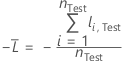
For a given tree in the forest, a class vote for a row in the test set is the predicted class for the row from the single tree. The predicted class for a row in test set is the class with the highest vote across all trees in the forest. The predicted class probability for a row in the test set is the ratio of the number of votes for the class and the total votes for the row. The likelihood calculations follow from these probabilities:
where

Notation for test set
| Term | Description |
|---|---|
| nTest | sample size of the test set |
| yi, Test | binary response value of case i in the test set. yi, k = 1 for event class, and 0 otherwise. |
 | predicted event probability for case i in the test set |
Area under ROC curve
Formula


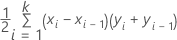
where k is the number of distinct event probabilities and (x0, y0) is the point (0, 0).
To compute the area for a curve from out-of-bag data or a test set, use the points from the corresponding curve.
Notation
| Term | Description |
|---|---|
| TPR | true positive rate |
| FPR | false positive rate |
| TP | true positive, events that were correctly assessed |
| FN | false negative, events that were incorrectly assessed |
| P | number of actual positive events |
| FP | false positive, nonevents that were incorrectly assessed |
| N | number of actual negative events |
| FNR | false negative rate |
| TNR | true negative rate |
Example
| x (false positive rate) | y (true positive rate) |
|---|---|
| 0.0923 | 0.3051 |
| 0.4154 | 0.7288 |
| 0.7538 | 0.9322 |
| 1 | 1 |


95% CI for the area under the ROC curve
The following interval gives the upper and lower bounds for the confidence interval:

The computation of the standard error of the area under the ROC curve
( )
comes from Salford Predictive Modeler®. For general information
about estimation of the variance of the area under the ROC curve, see the
following references:
)
comes from Salford Predictive Modeler®. For general information
about estimation of the variance of the area under the ROC curve, see the
following references:
Engelmann, B. (2011). Measures of a ratings discriminative power: Applications and limitations. In B. Engelmann & R. Rauhmeier (Eds.), The Basel II Risk Parameters: Estimation, Validation, Stress Testing - With Applications to Loan Risk Management (2nd ed.) Heidelberg; New York: Springer. doi:10.1007/978-3-642-16114-8
Cortes, C. and Mohri, M. (2005). Confidence intervals for the area under the ROC curve. Advances in neural information processing systems, 305-312.
Feng, D., Cortese, G., & Baumgartner, R. (2017). A comparison of confidence/credible interval methods for the area under the ROC curve for continuous diagnostic tests with small sample size. Statistical Methods in Medical Research, 26(6), 2603-2621. doi:10.1177/0962280215602040
Notation
| Term | Description |
|---|---|
| A | area under the ROC curve |
 | 0.975 percentile of the standard normal distribution |
Lift
To see general calculations for cumulative lift, go to Methods and formulas for the cumulative lift chart for Random Forests® Classification.
Misclassification rate
The following equation gives the misclassification rate:

The misclassed count is the number of rows in the out-of-bag data where their predicted classes are different from their true classes. Total count is the total number of rows in the out-of-bag data.
For validation with a test data set, the misclassed count is the sum of misclassifications in the test set. Total count is the number of rows in the test data set.