In This Topic
Null hypothesis, Alternative hypothesis
The test for equal variances is a hypothesis test that evaluates two mutually exclusive statements about two or more population standard deviations. These two statements are called the null hypothesis and the alternative hypotheses. A hypothesis test uses sample data to determine whether to reject the null hypothesis.
- Null hypothesis (H0)
- The null hypothesis states that the population standard deviations are all equal.
- Alternative hypothesis (HA)
- The alternative hypothesis states that not all population standard deviations are equal.
Interpretation
Compare the p-value to the significance level to determine whether to reject the null hypothesis.
N
The sample size (N) is the total number of observations in each group.
Interpretation
The sample size affects the confidence interval and the power of the test.
Usually, a larger sample yields a narrower confidence interval. A larger sample size also gives the test more power to detect a difference.
Standard Deviation (StDev)
The standard deviation is the most common measure of dispersion, or how spread out the data are around the mean. The symbol σ (sigma) is often used to represent the standard deviation of a population. The symbol s is used to represent the standard deviation of a sample.
Interpretation
The standard deviation uses the same units as the variable. A higher standard deviation value indicates greater spread in the data. A guideline for data that follow the normal distribution is that approximately 68% of the values fall within one standard deviation of the mean, 95% of the values fall within two standard deviations, and 99.7% of the values fall within three standard deviations.
Bonferroni confidence intervals
Use the Bonferroni confidence intervals to estimate the standard deviation of each population based on your categorical factors. Each confidence interval is a range of likely values that are likely to contain the standard deviation of the corresponding population. Minitab adjusts the Bonferroni confidence intervals to maintain the simultaneous confidence level.
Controlling the simultaneous confidence level is especially important when you assess multiple confidence intervals. If you do not control the simultaneous confidence level, the chance that at least one confidence interval does not contain the true standard deviation increases with the number of confidence intervals.
For more information, go to Understanding individual and simultaneous confidence levels in multiple comparisons and What is the Bonferroni method?.
Note
You cannot use these Bonferroni confidence intervals to determine whether the differences between pairs of groups are statistically significant. Use the p-values and the multiple comparisons confidence intervals on the summary plot to determine the statistical significance of the differences.
Interpretation
Method
| Null hypothesis | All variances are equal |
|---|---|
| Alternative hypothesis | At least one variance is different |
| Significance level | α = 0.05 |
95% Bonferroni Confidence Intervals for Standard Deviations
| Fertilizer | N | StDev | CI |
|---|---|---|---|
| GrowFast | 50 | 4.28743 | (3.43659, 5.61790) |
| None | 50 | 5.09137 | (4.24793, 6.40914) |
| SuperPlant | 49 | 5.49969 | (4.48577, 7.08914) |
In these results, the 95% Bonferroni confidence intervals indicate that you can be 95% confidence that the entire set of confidence intervals includes the true population standard deviations for all groups. Also, the individual confidence level indicates how confident you can be that an individual confidence interval contains the population standard deviation of that specific group. For example, you can be 98.3333% confident that the standard deviation for the GrowFast population is within the confidence interval (3.43659, 5.61790).
Individual confidence level
The individual confidence level is the percentage of times that a single confidence interval includes the true standard deviation for that specific group if you repeat the study multiple times.
As you increase the number of confidence intervals in a set, the chance that at least one confidence interval does not contain the true standard deviation increases. The simultaneous confidence level indicates how confident you can be that the entire set of confidence intervals includes the true population standard deviations for all groups.
Interpretation
Method
| Null hypothesis | All variances are equal |
|---|---|
| Alternative hypothesis | At least one variance is different |
| Significance level | α = 0.05 |
95% Bonferroni Confidence Intervals for Standard Deviations
| Fertilizer | N | StDev | CI |
|---|---|---|---|
| GrowFast | 50 | 4.28743 | (3.43659, 5.61790) |
| None | 50 | 5.09137 | (4.24793, 6.40914) |
| SuperPlant | 49 | 5.49969 | (4.48577, 7.08914) |
You can be 98.3333% confident that each individual confidence interval contains the population standard deviation for that specific group. For example, you can be 98.3333% confident that the standard deviation for the GrowFast population is within the confidence interval (3.43659, 5.61790). However, because the set includes three confidence intervals, you can be only 95% confident that all the intervals contain the true values.
Tests
The types of tests for equal variances that Minitab displays depends on whether you selected Use test based on normal distribution in the Options subdialog and the number of groups in your data.
Multiple comparisons, Levene's methods
If you did not select Use test based on normal distribution, Minitab displays test results for both the multiple comparisons method and Levene's method. For most continuous distributions, both methods give you a type 1 error rate that is close to your significance level (denoted as α or alpha). The multiple comparisons method is usually more powerful. If the p-value for the multiple comparisons method is significant, you can use the summary plot to identify specific populations that have standard deviations that are different from each other.
- Each of your samples has fewer than 20 observations.
- The distribution for one or more of the populations is extremely skewed or has heavy tails. Compared to the normal distribution, a distribution with heavy tails has more data at its lower and upper ends.
If the p-value for the multiple comparisons test is less than your chosen significance level, the differences between some of the standard deviations are statistically significant. Use the multiple comparison intervals to determine which standard deviations are significantly different from each other. If two intervals do not overlap, then the corresponding standard deviations (and variances) are significantly different.
When you have small samples from very skewed, or heavy-tailed distributions, the type I error rate for the multiple comparisons method can be higher than α. Under these conditions, if Levene's method gives you a smaller p-value than the multiple comparisons method, base your conclusions on Levene's method.
F-test, Bartlett's test
If you select Use test based on normal distribution and you have two groups, Minitab performs the F-test. If you have 3 or more groups, Minitab performs Bartlett's test.
The F-test and Bartlett's test are accurate only for normally distributed data. Any departure from normality can cause these tests to yield inaccurate results. However, if the data conform to the normal distribution, the F-test and Bartlett's test are typically more powerful than either the multiple comparisons method or Levene's method.
If the p-value for the test is less than your significance level, the differences between some of the standard deviations are statistically significant.
Test Statistic
Note
The multiple comparisons test does not use a test statistic.
Interpretation
Minitab uses the test statistic to calculate the p-value, which you use to make a decision about the statistical significance of the differences between standard deviations. The p-value is a probability that measures the evidence against the null hypothesis. Lower probabilities provide stronger evidence against the null hypothesis.
A sufficiently high test statistic indicates that the difference between some of the standard deviations is statistically significant.
You can use the test statistic to determine whether to reject the null hypothesis. However, the p-value is used more often because it is easier to interpret.
P-value
The p-value is a probability that measures the evidence against the null hypothesis. Lower probabilities provide stronger evidence against the null hypothesis.
Interpretation
Use the p-value to determine whether any of the differences between the standard deviations are statistically significant. Minitab displays the results of either one or two tests that assess the equality of variances. If you have two p-values and they disagree, see "Tests".
To determine whether any of the differences between the standard deviations are statistically significant, compare the p-value to your significance level to assess the null hypothesis. The null hypothesis states that the group means are all equal. Usually, a significance level (denoted as α or alpha) of 0.05 works well. A significance level of 0.05 indicates a 5% risk of concluding that a difference exists when there is no actual difference.
- If the p-value is > α, the differences between the standard deviations are not statistically significant.
- If the p-value is ≤ α, the differences between some of the standard deviations are statistically significant.
Summary plot
The summary plot shows p-values and confidence intervals for the equal variances tests. The types of tests and intervals that Minitab displays depend on whether you selected Use test based on normal distribution in the Options dialog box and on the number of groups in your data.
If you did not select Use test based on normal distribution, the summary plot displays p-values for both the multiple comparisons method and Levene's method. The plot also displays multiple comparison intervals. You must choose between the two methods based on the properties of your data.
If you selected Use test based on normal distribution and have two groups, Minitab performs the F-test. If you have 3 or more groups, Minitab performs Bartlett's test. For either of these tests, the plot also displays Bonferroni confidence intervals.
P-values
The p-value is a probability that measures the evidence against the null hypothesis. Lower probabilities provide stronger evidence against the null hypothesis.
Use the p-values to determine whether any of the differences between the standard deviations are statistically significant. Minitab displays the results of either one or two tests that assess the equality of variances. If you have two p-values and they disagree, see the section on Tests for information about which test to use.
To determine whether any of the differences between the standard deviations are statistically significant, compare the p-value to your significance level to assess the null hypothesis. The null hypothesis states that the group standard deviations are all equal. Usually, a significance level (denoted as α or alpha) of 0.05 works well. A significance level of 0.05 indicates a 5% risk of concluding that a difference exists when there is no actual difference.
- If the p-value is > α, the differences between the standard deviations are not statistically significant.
- If the p-value is ≤ α, the differences between some of the standard deviations are statistically significant.
Multiple comparison intervals
If you did not select Use test based on normal distribution, the summary plot displays multiple comparison intervals.
If it is valid for you to use the multiple comparison p-value, you can use the multiple comparison confidence intervals to identify specific pairs of groups which have a difference that is statistically significant. If two intervals do not overlap, the difference between the corresponding standard deviations is statistically significant.
If the properties of your data require that you use Levene's method, do not assess the confidence intervals on the summary plot.
Bonferroni confidence intervals
If you selected Use test based on normal distribution, the summary plot displays Bonferroni confidence intervals.
Use the Bonferroni confidence intervals to estimate the standard deviation of each population for your categorical factors. Each confidence interval is a range of values that is likely to contain the standard deviation of the corresponding population. Minitab adjusts the Bonferroni confidence intervals to control the simultaneous confidence level.
Controlling the simultaneous confidence level is especially important when you assess multiple confidence intervals. If you do not control the simultaneous confidence level, the chance that at least one confidence interval does not contain the true standard deviation increases with the number of confidence intervals.
For more information, go to Understanding individual and simultaneous confidence levels in multiple comparisons and What is the Bonferroni method?
Note
You cannot use these Bonferroni confidence intervals to determine whether the differences between pairs of groups are statistically significant. Use the p-values and the multiple comparisons confidence intervals on the summary plot to determine the statistical significance of the differences.
Interpretation
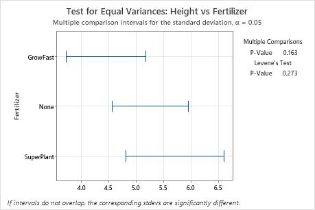
In this summary plot, the p-value for the multiple comparisons test is higher than the significance level of 0.05. None of the differences between the groups are statistically significant, and all the multiple comparison intervals overlap.
Individual value plot
An individual value plot displays the individual values in each sample. The individual value plot makes it easy to compare the samples. Each circle represents one observation. An individual value plot is especially useful when your sample size is small.
Interpretation
Use an individual value plot to examine the spread of the data and to identify any potential outliers. Individual value plots are best when the sample size is less than 50.
- Skewed data
-
Examine the spread of your data to determine whether your data appear to be skewed. When data are skewed, the majority of the data are located on the high or low side of the graph. Skewed data indicate that the data might not be normally distributed. Often, skewness is easiest to detect with an individual value plot, a histogram, or a boxplot.
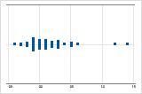
Right-skewed
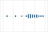
Left-skewed
The individual value plot with right-skewed data shows wait times. Most of the wait times are relatively short, and only a few wait times are longer. The individual value plot with left-skewed data shows failure time data. A few items fail immediately, and many more items fail later.
- Outliers
-
Outliers, which are data values that are far away from other data values, can strongly affect your results. Often, outliers are easy to identify on an individual value plot.
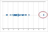
On an individual value plot, unusually low or high data values indicate potential outliers.
Try to identify the cause of any outliers. Correct any data-entry errors or measurement errors. Consider removing data values for abnormal, one-time events (special causes). Then, repeat the analysis.
Boxplot
A boxplot provides a graphical summary of the distribution of each sample. The boxplot makes it easy to compare the shape, the central tendency, and the variability of the samples.
Interpretation
Use a boxplot to examine the spread of the data and to identify any potential outliers. Boxplots are best when the sample size is greater than 20.
- Skewed data
-
Examine the spread of your data to determine whether your data appear to be skewed. When data are skewed, the majority of the data are located on the high or low side of the graph. Skewed data indicates that the data might not be normally distributed. Often, skewness is easiest to detect with an individual value plot, a histogram, or a boxplot.
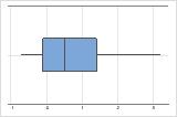
Right-skewed
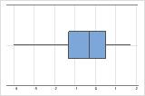
Left-skewed
The boxplot with right-skewed data shows average wait times. Most of the wait times are relatively short, and only a few of the wait times are longer. The boxplot with left-skewed data shows failure rate data. A few items fail immediately, and many more items fail later.
Data that are severely skewed can affect the validity of the p-value if your sample is small (< 20 values). If your data are severely skewed and you have a small sample, consider increasing your sample size.
- Outliers
-
Outliers, which are data values that are far away from other data values, can strongly affect your results. Often, outliers are easiest to identify on a boxplot.
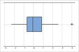
On a boxplot, asterisks (*) denote outliers.
Try to identify the cause of any outliers. Correct any data-entry errors or measurement errors. Consider removing data values for abnormal, one-time events (special causes). Then, repeat the analysis.