In This Topic
Significance level (α)
The significance level (denoted by alpha or α) is the maximum acceptable level of risk for a type I error.
Interpretation
Use the significance level to decide whether a difference is statistically significant. Because the significance level is the threshold for statistical significance, a higher value increases the chance of making a type I error. A type I error is the incorrect conclusion that a difference exists between the means at different factor levels.
Assumed standard deviation
The assumed standard deviation is the estimate of the standard deviation of the response measurements at replicated experimental runs. If you already performed an analysis in minitab that produced an ANOVA table, you can use the square root of the adjusted mean square for error.
Interpretation
Use the assumed standard deviation to describe how variable the data are. Higher values of the assumed standard deviation indicate more variation or "noise" in the data, which decreases the statistical power of a design.
Factors
The number shows how many factors are in the design.
Interpretation
Use the number of factors to verify that the design has all of the factors that you need to study. Factors are the variables that you control in the experiment. Factors are also known as independent variables, explanatory variables, and predictor variables. Factors can assume only a limited number of possible values, known as factor levels. For a general full factorial design, all factors are categorical.
For example, you are studying factors that could affect plastic strength during the manufacturing process. You decide to include Additive in your experiment. The additive is a categorical variable that can be type A or type B.
Number of levels
The list shows the number of levels in each factor that is in the design.
Interpretation
Use the number of levels to verify that the design has all the factors that you need to study. For example, you are studying factors that could affect plastic strength during the manufacturing process. You decide to include a factor about an additive. The additive is a categorical variable. The additive can b either type A or type B. The number of levels for the factor for additive is 2.
Include terms in the model up through order
The model order is the highest order of interaction that Minitab uses to determine the number of terms.
Interpretation
Use the model order to verify the model that the power calculations assume. For example, to study an interaction between 3 factors, the model order can be 3 or more.
The higher the order, the more terms are in the model. Models with more terms have fewer degrees of freedom for error. Thus, designs with more terms have lower power than designs with fewer terms when all other properties are the same. If you perform a calculation where the model order is the same as the number of factors, then the calculations require more than one replicate.
In these results, the power calculations are for the model with terms up through order 3. The number of factors is also 3. Because this model uses all degrees of freedom from a single replicate of the design, Minitab does not calculate power for a single replicate. If you perform the same calculation for terms up through order 2, you can calculate power for 1 replicate.
Results
| Maximum Difference | Reps | Total Runs | Power |
|---|---|---|---|
| 2 | 3 | 108 | 0.930642 |
| 3 | 3 | 108 | 0.999667 |
Maximum difference
The maximum difference is the difference that you want to detect between the factor levels that have the highest and lowest means. The calculations use the factor that has the most levels to produce calculations that are conservative for other factors. Minitab calculates the smallest difference that the design detects. More replicates give the design the ability to detect smaller differences. Usually, you want to be able to detect the smallest difference that has practical consequences for your application.
Interpretation
Use the maximum difference to determine what differences the designed experiment detects. If you enter a number of replicates and a power value, then Minitab calculates the maximum difference. Usually, more replicates let you detect a smaller maximum difference. Usually, the more replicates, the smaller the maximum difference the designed experiment detects.
In these results, the design with one replicate can detect a difference of about 3.8 with 90% power. The design with 3 replicates can detect a smaller difference with 90% power, about 1.9.
These results also show that the factor with the most levels has 4 levels. The calculated maximum difference is accurate for the 4-level factor. The maximum difference for the 4-level factor is larger than the maximum difference for the two 3-level factors.
Results
| Reps | Total Runs | Power | Maximum Difference |
|---|---|---|---|
| 1 | 36 | 0.9 | 3.77758 |
| 3 | 108 | 0.9 | 1.88781 |
Reps
Replicates are multiple experimental runs with the same factor settings.
Interpretation
Use the number of replicates to estimate how many experimental runs to include in the design. If you enter a power and maximum difference, Minitab calculates the number of replicates. Because the numbers of replicates are given in integer values, the actual power may be greater than your target value. If you increase the number of replicates, the power of your design also increases. You want enough replicates to achieve adequate power.
Because the replicates are integer values, the power values that you specify are target power values. The actual power values are for the number of replicates and the number of center points in the designed experiment. The actual power values are at least as large as the target power values.
In these results, Minitab calculates the number of replicates to reach a target power of 80% and a target power of 90%. To detect a difference of 2.0, the design requires 3 replicates to achieve either the target of 80% or the target of 90%. The power for the design with 2 replicates is less than the target power of 80%. To detect the smaller difference of 1.8, 3 replicates gives more than 80% power but not more than 90% power. To detect the smaller difference with 90% power, the designed experiment needs 4 replicates. Because the numbers of replicates are integers, the actual powers are greater than the target powers.
These results also show that the factor with the most levels has 4 levels. These results are accurate for the 4-level factor. The number of replicates could be different for the two 3-level factors, especially if the actual power is much greater than the target power.
Results
| Maximum Difference | Reps | Total Runs | Target Power | Actual Power |
|---|---|---|---|---|
| 2.0 | 3 | 108 | 0.8 | 0.932615 |
| 2.0 | 3 | 108 | 0.9 | 0.932615 |
| 1.8 | 3 | 108 | 0.8 | 0.867493 |
| 1.8 | 4 | 144 | 0.9 | 0.952918 |
Total Runs
An experimental run is a factor level combination at which you measure responses. The total number of runs is how many measurements of the response are in the design. Multiple executions of the same factor level combination are considered separate experimental runs and are called replicates.
Interpretation
Use the number of total runs to verify that the designed experiment is the right size for your resources. For a general full factorial design, this formula gives the total number of runs:

| Term | Description |
|---|---|
| n | Number of replicates |
| Li | Number of levels in the ith factor |
| k | Number of factors |
In these results, the experiment has one 4-level factor and two 3-level factors. The number of runs in a single replicate is 4*3*3 = 36. Each replicate adds the same number of runs. Thus, the number of runs in 3 replicates of a 36-experimental run design is 36*3 = 108. Experiments with more experimental runs have more power to detect a difference.
Results
| Maximum Difference | Reps | Total Runs | Power |
|---|---|---|---|
| 2.5 | 1 | 36 | 0.539953 |
| 2.5 | 3 | 108 | 0.992993 |
Power
The power of a general full factorial design is the probability that the main effect for the factor with the most levels is statistically significant. The difference is between the greatest and least means of the response variable for the factor with the most levels. Power calculations are conservative for factors with fewer levels that are in the same design.
Interpretation
Use the power value to determine the ability of the design to detect a difference. If you enter a number of replicates and a maximum difference, then Minitab calculates the power of the design. A power value of 0.9 is usually considered adequate. A value of 0.9 indicates that you have a 90% chance of detecting the difference between the factor levels if the difference is the size that you specify. Usually, when the number of replicates is smaller, the power is lower. If a design has low power, you can fail to detect a difference and mistakenly conclude that none exists.
These results demonstrate how an increase in the number of replicates increases the power. For a difference of 2, the power of the design is approximately 0.36 with 1 replicate. With 3 replicates, the power increases to approximately 0.93.
These results also demonstrate how an increase in the effect size increases the power. For a design with 1 replicate and a difference of 2, the power is approximately 0.36. For a design with 1 replicate and a difference of 3, the power is approximately 0.71.
Results
| Maximum Difference | Reps | Total Runs | Power |
|---|---|---|---|
| 2 | 1 | 36 | 0.362893 |
| 2 | 3 | 108 | 0.932615 |
| 3 | 1 | 36 | 0.712094 |
| 3 | 3 | 108 | 0.999695 |
Power curve
The power curve plots the power of the test versus the maximum difference. Maximum difference refers to the difference between the greatest and least means for the factor with the most levels. Power calculations are conservative for factors with fewer levels that are in the same design.
Interpretation
Use the power curve to assess the appropriate properties for your design.
The power curve represents the relationship between power and maximum difference for each number of replicates. Each symbol on the power curve represents a calculated value based on the properties that you enter. For example, if you enter a number of replicates and a power value, Minitab calculates the corresponding maximum difference and displays the calculated value on the graph.
Examine the values on the curve to determine the difference between the largest and smallest means for the factor with the most levels that the experiment detects at a certain power value and number of replicates. A power value of 0.9 is usually considered adequate. However, some practitioners consider a power value of 0.8 to be adequate. If a design has low power, you might fail to detect a difference that is practically significant. Increasing the total number of experimental runs increases the power of your design. You want enough experimental runs in your design to achieve adequate power. A design has more power to detect a larger difference than a smaller difference.
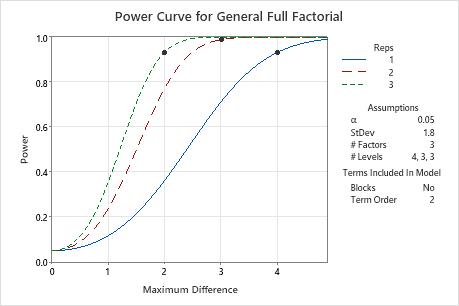
In these results, Minitab calculates the number of replicates to achieve a power of at least 0.9 for maximum differences of 2, 3 or 4. The plot has a curve for each number of replicates. To detect a maximum difference of 2 with a power of at least 0.9, the design needs 3 replicates. The plot contains a curve for 3 replicates and shows a symbol at a maximum difference of 2 where the power exceeds 0.9. To detect a maximum difference of 3 with at least 0.9 power, the design needs 2 replicates. For a maximum difference of 4 with at least 0.9 power, the design needs 1 replicate.
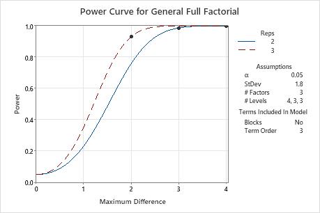
Compare the power curve for a term order of 3 to the power curve for a term order of 2. The solution with 1 replicate is possible only when the term order is less than the number of factors. If the number of factors equals the term order, a 1-replicate design does not have enough degrees of freedom for power calculations. In the results the term order is 3 and the number of factors is 3, so the 1-replicate design is not a possible solution. The solution when the maximum difference is 4 becomes the 2-replicate design.