A quality engineer at a consumer electronics company wants to know whether the defects per television set are from a Poisson distribution. The engineer randomly selects 300 televisions and records the number of defects per television.
- Open the sample data, TelevisionDefects.MWX.
- Choose .
- In Variable, enter Defects.
- In Frequency variable: (optional), enter Observed.
- Click OK.
Interpret the results
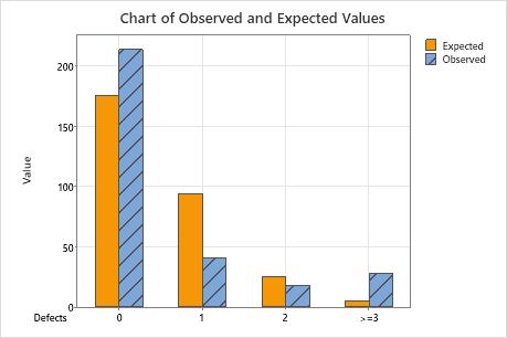
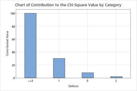
The null hypothesis states that the data follow a Poisson distribution. Because the p-value is 0.000, which is less than the significance level of 0.05, the engineer rejects the null hypothesis and concludes that the data do not follow a Poisson distribution. The graphs indicate that the difference between the observed and expected values is large for categories 1 and  3, and that category 3 is the highest contributor to the chi-square statistic.
Method
| Frequencies in Observed |
|---|
Descriptive Statistics
| N | Mean |
|---|---|
| 300 | 0.536667 |
Observed and Expected Counts for Defects
| Defects | Poisson Probability | Observed Count | Expected Count | Contribution to Chi-Square |
|---|---|---|---|---|
| 0 | 0.584694 | 213 | 175.408 | 8.056 |
| 1 | 0.313786 | 41 | 94.136 | 29.993 |
| 2 | 0.084199 | 18 | 25.260 | 2.086 |
| >=3 | 0.017321 | 28 | 5.196 | 100.072 |
Chi-Square Test
| Null hypothesis | H₀: Data follow a Poisson distribution |
|---|---|
| Alternative hypothesis | H₁: Data do not follow a Poisson distribution |
| DF | Chi-Square | P-Value |
|---|---|---|
| 2 | 140.208 | 0.000 |