In This Topic
Optimization plot
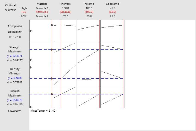
The optimization plot shows how the variables affect the predicted responses. Double-click the optimization plot to make it interactive and investigate how the variables affect the predicted responses.
When the optimization plot is interactive, the cells show how the corresponding response variable or composite desirability changes as a function of one of the variables, while all other variables remain fixed.
- Column for each variable (predictor)
- The vertical red lines on the graph represent the current settings.
- Row for each response variable.
- The horizontal blue lines represent the current response values.
- Composite desirability
- In the top row and in the upper left corner, is the composite desirability (D).
- Interactive toolbar
- The Predict button in the top left of the toolbar calculates the prediction for the current variable settings.
The type of fitted values that Minitab displays depends on the type of response variable in your model. For instance, Minitab displays means, probabilities, or standard deviations depending on whether you have continuous or count measurements, binary data, or models that use Analyze Variability.
The optimization plot displays the fitted values for the predictor settings. However, you should examine prediction intervals to determine whether the range of likely values for a single future value falls within acceptable boundaries for the process.
Interpretation
Use the optimization plot to determine the optimal settings for the predictors given the parameters that you specified.
- Material: The two points for each cell in this column represent the two levels of the categorical variable: Formula1 and Formula2. Formula2 appears to be the best material. Changing to Formula1 would decrease the insulative value and increase the density, which are both undesirable. However, because material type interacts with other factors, this trend might not hold at other settings. Consider whether you can find a local solution for Formula1. Or, change the settings for Formula1 directly on the graph by moving the vertical bars.
- InjPress: Increasing the injection pressure increases all three responses. Therefore, the optimal setting is in the middle of the range (98.4848), which is a compromise between conflicting goals. The goal is to maximize insulative value, minimize density, and maximize strength.
- InjTemp: Increasing injection temperature also increases all the responses. But the effect on density is minimal compared to the effect on insulative value. Therefore, you increase the composite desirability by maximizing the injection temperature. The optimal settings of injection temperature are at the maximum levels in the experiment. This result suggests that you should consider experimenting with higher temperatures.
- CoolTemp: Increasing cooling temperature increases insulative value, but decreases both density and strength. The optimal settings of both injection temperature and cooling temperature are at the maximum levels in the experiment. This result suggests that you should consider experimenting with higher temperatures. The graphs show that higher cooling temperatures may be especially worth considering. If the graphs could be extrapolated, higher cooling temperatures would improve insulative value and density. However, strength would decrease.
Parameters
Minitab displays the design parameters for each response in the Parameters table. Examine these results to verify that the displayed design parameters are correct.
Your choices of goal, lower, target, upper, and weight define the desirability function for each individual response. The importance parameters determine how the desirability functions are combined into a single composite desirability.
Interpretation
- The goal for Strength is to maximize it. A value of 38.1821 is considered excellent, and values below 19.2189 are unacceptable.
- The goal for Density is to minimize it. A value of 0.4351 is considered excellent, and values above 1.60314 are unacceptable.
- The goal for Insulation is to maximize it. A value of 27.7156 is considered excellent, and values below 13.2905 are unacceptable.
All three responses have the same importance value. Therefore, all three responses have an equal influence on the composite desirability.
Multiple Response Prediction
| Variable | Setting |
|---|---|
| Material | Formula2 |
| InjPress | 98.4848 |
| InjTemp | 100 |
| CoolTemp | 45 |
| MeasTemp | 21.4875 |
| Response | Fit | SE Fit | 95% CI | 95% PI |
|---|---|---|---|---|
| Strength | 32.34 | 1.04 | (29.45, 35.22) | (27.25, 37.43) |
| Density | 0.6826 | 0.0597 | (0.5167, 0.8484) | (0.3899, 0.9753) |
| Insulation | 25.608 | 0.268 | (24.863, 26.352) | (24.294, 26.921) |
Multiple response prediction
Minitab uses the variable settings in this table to calculate the fits for all of the responses that are included in the optimization procedure.
When you first run Response Optimizer, the multiple response prediction table displays the optimal values that the algorithm identifies. If you change the variable settings on the graph and click the Predict button on the toolbar, then Minitab makes a table with the new settings.
Use this table to verify that you performed the analysis as you intended.
Fit
Fitted values are also called fits or  . The fitted values are point estimates of the mean response for given values of the predictors. The values of the predictors are also called x-values. Minitab uses the regression equation and the variable settings to calculate the fit.
The type of fitted values that Minitab displays depends on the type of response variable in your model. For instance, Minitab displays means, probabilities, or standard deviations depending on whether you have continuous or count measurements, binary data, or models that use Analyze Variability.
Interpretation
Fitted values are calculated by entering x-values into the model equation for a response variable.
For example, if the equation is y = 5 + 10x, the fitted value for the x-value, 2, is 25 (25 = 5 + 10(2)).
SE Fit
The standard error of the fit (SE fit) estimates the variation in the estimated mean response for the specified variable settings. The calculation of the confidence interval for the mean response uses the standard error of the fit. Standard errors are always non-negative.
Interpretation
Use the standard error of the fit to measure the precision of the estimate of the mean response. The smaller the standard error, the more precise the predicted mean response. For example, an analyst develops a model to predict delivery time. For one set of variable settings, the model predicts a mean delivery time of 3.80 days. The standard error of the fit for these settings is 0.08 days. For a second set of variable settings, the model produces the same mean delivery time with a standard error of the fit of 0.02 days. The analyst can be more confident that the mean delivery time for the second set of variable settings is close to 3.80 days.
With the fitted value, you can use the standard error of the fit to create a confidence interval for the mean response. For example, depending on the number of degrees of freedom, a 95% confidence interval extends approximately two standard errors above and below the predicted mean. For the delivery times, the 95% confidence interval for the predicted mean of 3.80 days when the standard error is 0.08 is (3.64, 3.96) days. You can be 95% confident that the population mean is within this range. When the standard error is 0.02, the 95% confidence interval is (3.76, 3.84) days. The confidence interval for the second set of variable settings is narrower because the standard error is smaller.
95% CI
The confidence interval for the fit provides a range of likely values for the mean response given the specified settings of the predictors.
Interpretation
Use the confidence interval to assess the estimate of the fitted value for the observed values of the variables.
For example, with a 95% confidence level, you can be 95% confident that the confidence interval contains the population mean for the specified values of the variables in the model. The confidence interval helps you assess the practical significance of your results. Use your specialized knowledge to determine whether the confidence interval includes values that have practical significance for your situation. A wide confidence interval indicates that you can be less confident about the mean of future values. If the interval is too wide to be useful, consider increasing your sample size.
95% PI
The prediction interval is a range that is likely to contain a single future response for a selected combination of variable settings.
Interpretation
Use the prediction intervals (PI) to assess the precision of the predictions. The prediction intervals help you assess the practical significance of your results. If a prediction interval extends outside of acceptable boundaries, the predictions might not be sufficiently precise for your requirements.
With a 95% PI, you can be 95% confident that a single response will be contained in the interval given the settings of the predictors that you specified. The prediction interval is always wider than the confidence interval because of the added uncertainty involved in predicting a single response versus the mean response.
For example, a materials engineer at a furniture manufacturer develops a simple regression model to predict the stiffness of particleboard from the density of the board. The engineer verifies that the model meets the assumptions of the analysis. Then, the analyst uses the model to predict the stiffness.
The regression equation predicts that the stiffness for a new observation with a density of 25 is -21.53 + 3.541*25, or 66.995. Although such an observation is unlikely to have a stiffness of exactly 66.995, the prediction interval indicates that the engineer can be 95% confident that the actual value will be between approximately 48 and 86.
Composite desirability
Use composite desirability (D) to evaluate how well the settings optimize a set of responses overall. Desirability has a range of zero to one. One represents the ideal case; zero indicates that one or more responses are outside their acceptable limits.
Often, if you have multiple responses, there is no factor setting that simultaneously maximizes the desirability of all the responses. For this reason, Minitab maximizes the composite desirability. The composite desirability combines the individual desirability of all the response variables into a single measure. Greater emphasis is placed on the response variables with the greatest importance.
For more information, read What are individual desirability and composite desirability?.
Interpretation
Composite desirability values that are close to 1 indicate that the settings achieve favorable results for all responses.