In This Topic
Step 1: Look for evidence of autocorrelation
To look for evidence of autocorrelation in the two series, examine the cross-correlation function for a large correlation, with the correlations on both sides slowly decreasing to 0. The autocorrelation usually causes difficulty in identifying meaningful relationships between the two time series. If you see evidence of autocorrelation, you should pre-whiten the data. For more information, go to Pre-whitening data for the cross-correlation function.
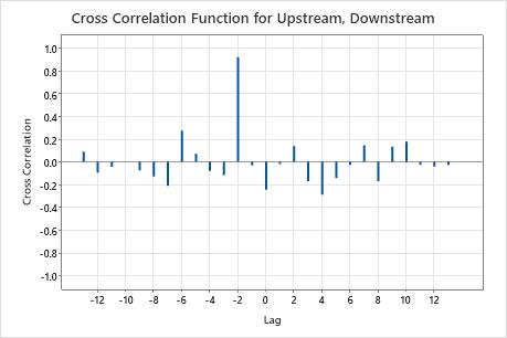
This plot shows that there is a large correlation, but the correlations on both sides do not slowly decrease to 0. The plot does not show any evidence of autocorrelation.
Step 2: Determine whether a relationship exists between the two series
To determine whether a relationship exists between the two series, look for a large correlation, with the correlations on both sides that quickly become non-significant. Usually, a correlation is significant when the absolute value is greater than  , where n is the number of observations and k is the lag. This calculation is a rule of thumb procedure based on large-sample normal approximation. If the population cross correlation of lag k is zero for k=1, 2 ... then, for fairly large n, rxy(k) will be approximately normally distributed, with mean (μ) zero and standard deviation (σ) 1/
 . Since approximately 95% of a normal population is within 2 standard deviations of the mean, a test that rejects the hypothesis that the population cross correlation of lag k equals zero when |rxy(k) | is greater than 2/
 has a significance level (α) of approximately 5%.
On this plot, the correlation at lag −2 is approximately 0.92. Because 0.92 > 0.5547 =  the correlation is significant. You can conclude that the water moves from the upstream location to the downstream location in two days.