In This Topic
X-scores
The x-scores are linear combinations of the terms; similar to principal component scores. The x-scores form an n × m matrix of uncorrelated columns. The x-scores are projections of the observations on the PLS components. PLS fits the x-scores, which replace the original terms in the data, using least squares estimation.
Formula

Notation
| Term | Description |
|---|---|
| n | the number of observations |
| m | the number of components |
| i | the observations from 1 to n |
| j | the terms from 1 to p |
| X | the design matrix |
| W | the x-weight matrix |
X-loadings
The x-loadings are linear coefficients that link the terms to the x-scores; similar to eigenvectors in principal components analysis. The loading values indicate the importance of the corresponding term to the mth component. The x-loadings form a p × m matrix.
Formula

Notation
| Term | Description |
|---|---|
| p | the number of terms |
| m | the number of components |
| i | the observations from 1 to n |
| j | the terms from 1 to p |
| t | the x-scores |
| X | the predictors |
X-weights
The x-weights describe the covariance between the terms and the responses. In the algorithm, the weights ensure the x-scores are orthogonal, or unrelated to one another, and are used to calculate the x-scores. The x-weights form a p × m matrix.
Formula

Minitab scales the vector of weights so that the length of the vector is 1.
Notation
| Term | Description |
|---|---|
| p | the number of terms |
| m | the number of components |
| i | the observations from 1 to n |
| j | the terms from 1 to p |
| X | the x-residual matrix |
| u | the y-scores |
X-residuals
The x-residuals contain the variance in the predictors not explained by the PLS model. Observations with relatively large x-residuals are outliers in the x-space, indicating that they are not well explained by the model.
The x-residuals are the differences between the actual predictor values and the x-calculated values and are on the same scale as the original predictors. The x-residual matrix, similar to the original x-matrix, is an n × p matrix.
The x-residual matrix is initialized to the standardized x-matrix. After calculating the m th component and obtaining the x-score vector and the x-loading vector, Minitab calculates the x-residuals.
Formula

Minitab then calculates the unstandardized x-residuals by multiplying the standardized x-residuals by the standard deviation of the predictor values.
Notation
| Term | Description |
|---|---|
| n | the number of observations |
| p | the number of terms |
| i | the observations from 1 to n |
| j | the terms from 1 to p |
| t | the x-scores |
| l | the x-loadings |
X-calculated values
The x-calculated values are linear combinations of the x-scores; contain the variance in the predictors explained by the PLS model. Observations with relatively small x-calculated values are outliers in the x-space and are not well explained by the model.
The x-calculated matrix, similar to the original x-matrix, is an n × p matrix, where n equals the number of observations and p equals the number of predictors. The x-calculated values are on the same scale as the predictors.
The x-calculated matrix is initialized to the zero matrix. After calculating the m th component and obtaining the x-score vector and the x-loading vector, Minitab calculates the x-calculated values. If the number of components equals the number of predictors, then the x-calculated value equals the original x-value.
Formula

Minitab then calculates the unstandardized x-calculated values by multiplying the standardized x-calculated values by the standard deviation of the predictor values and adding the mean.
Notation
| Term | Description |
|---|---|
| n | the number of observations |
| p | the number of predictors |
| i | the number of observations from 1 to n |
| j | the number of predictors from 1 to p |
| t | the x-scores |
| l | the x-loadings |
Y-scores
The y-scores are linear combinations of the response variables. The y-scores form an n × m matrix. The y-scores are projections of the observations on the PLS components.
Formula

Notation
| Term | Description |
|---|---|
| n | the number of observations |
| m | the number of components |
| k | the number of responses from 1 to r |
| Y | the y matrix |
| c | the y-loadings |
Y-loadings
The y-loadings are linear coefficients that link the responses to the y-scores. The loading values indicate the importance of the corresponding response to the m th component. The y-loadings form an r ×m matrix.
Formula

Notation
| Term | Description |
|---|---|
| r | the number of responses |
| m | the number of components |
| i | the observations from 1 to n |
| k | the responses from 1 to r |
| Y | the responses |
| t | the x-scores |
Y-residuals
The y-residuals contain the remaining variance in the responses not explained by the PLS model. Observations with relatively large y-residuals are outliers in the y-space, indicating that they are not well explained.
The y-residuals are the differences between the actual response values and the y-calculated values, and are on the same scale as the original responses. The y-residual matrix, similar to the original y-matrix, is an n × r matrix.
The y-residual matrix is initially set to the standardized Y matrix. After Minitab calculates the m th component and obtains the x-score and y-loading vectors, Minitab determines the standardized y-residuals.
Formula

Minitab then calculates the unstandardized y-residuals by multiplying the standardized y-residuals by the standard deviation of the corresponding response values.
Notation
| Term | Description |
|---|---|
| n | the number of observations |
| r | the number of responses |
| i | the observations from 1 to n |
| k | the responses from 1 to r |
| t | the x-scores |
| c | the y-loadings |
Y-calculated values
The y-calculated values are linear combinations of the x-scores; contain the variance in the responses explained by the PLS model. Observations with relatively small y-calculated values are outliers in the y-space and are not well explained.
The y-calculated matrix, like the original y-matrix, is an n x r matrix. The y-calculated matrix is initially set to the zero matrix. After Minitab calculates the m th component and obtains the x-score and y-loading vectors, Minitab determines the standardized y-calculated values.
Formula
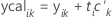
Minitab then calculates the unstandardized y-calculated values by multiplying the standardized y-calculated values by the standard deviation of the corresponding response and adding the mean.
Notation
| Term | Description |
|---|---|
| n | the number of observations |
| r | the number of responses |
| i | the observations from 1 to n |
| k | the responses from 1 to r |
| t | the x-scores |
| c | the y-loadings |