Select the method or formula of your choice.
In This Topic
Plotted points
Center line and control limits
Center line (CL)
The center line is the 50th percentile of the distribution. The center line equals G2 – 1.
Note
1 is subtracted because Minitab uses the "number until" definition of the geometric distribution in its calculations but plots the "number between" values on the G chart..
G2 equals INVCDF (0.5) for a geometric distribution with parameter p.
Minitab gives 2 values, G2a and G2b (G2a = G2b – 1), with 2 probabilities p2a and p2b (p2a < p2b). Using simple linear interpolation, G2 = G2a + (0.5 – p2a) / (p2b – p2a).
Lower control limit (LCL)
LCL = G1 – 1
G1 equals INVCDF (0.00135) for a geometric distribution with parameter p.
Minitab gives 2 values, G1a and G1b (G1a = G1b – 1), with 2 probabilities p1a and p1b (p1a < p1b). Using simple linear interpolation, G1 = G1a + (.00135 – p1a) / (p1b – p1a).
Upper control limit (UCL)
UCL = G3 – 1
G3 equals INVCDF (0.99865) for a geometric distribution with parameter p.
Minitab gives 2 values, G3a and G3b (G3a = G3b – 1), with 2 probabilities p3a and p3b (p3a < p3b). Using simple linear interpolation, we get G3 = G3a + (0.99865 – p3a) / (p3b – p3a).
Notation
| Term | Description |
|---|---|
| N | number of data values used in the calculations (If data are dates, subtract 1 because Minitab plots the differences.) |
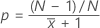
 | average of the plotted points |
| Event probability (p) |
 |
Tests for special causes, including Benneyan test
Tests 1−4
Test 1 is based on the geometric distribution. Tests 2, 3 and 4 are identical to the tests used in the attribute charts.
- G1 = INVCDF (0.00135) for a geometric distribution with parameter p
- G3 = INVCDF (0.99865) for a geometric distribution with parameter p; average of the plotted points
- G1' = INVCDF (p1') for a geometric distribution with parameter p
- G3' = INVCDF (p2') for a geometric distribution with parameter p
- p1' = CDF (–K) for a normal distribution with mean = 0 and standard deviation = 1
- p2' = CDF (K) for a normal distribution with mean = 0 and standard deviation = 1
Benneyan test
The Benneyan test counts the number of consecutive plotted points equal to the lower control limit using the following formula to generate a signal:
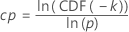
Minitab rounds cp up to the next integer and uses that value as the number of consecutive points equal to the lower control limit that are required to produce a signal.
See Benneyan1 for more information on the Benneyan test.
Notation
| Term | Description |
|---|---|
| CDF() | CDF for a normal distribution with mean 0, standard deviation 1 |
| k | parameter for Test 1. The default is 3. |