In This Topic
Histogram
A histogram divides sample values into many intervals and represents the frequency of data values in each interval with a bar.
Interpretation
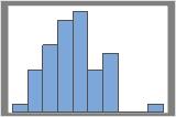
50 resamples
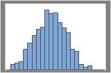
1000 resamples
The distribution is usually easier to determine with more resamples. For example, in these data, the distribution is ambiguous for 50 resamples. With 1000 resamples, the shape looks approximately normal.
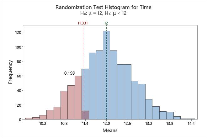
The histogram visually shows the results of the hypothesis test. Minitab adjusts the data so that the center of the resamples is the same as the hypothesized mean. For a one-sided test, a reference line is drawn at the mean of the original sample. For a two-sided test, a reference line is drawn at the mean of the original sample and at the same distance on the opposite side of the hypothesized mean. The p-value is the proportion of sample means that are more extreme than the values at the reference lines. In other words, the p-value is the proportion of sample means that are as extreme as your original sample when you assume that the null hypothesis is true. These means are colored red on the histogram.
In this histogram, the bootstrap distribution appears to be normal. The p-value of 0.2030 indicates that 20.3% of the sample means are less than the mean of the original sample.
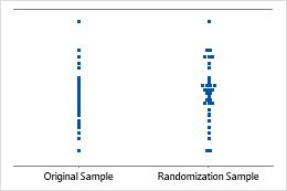
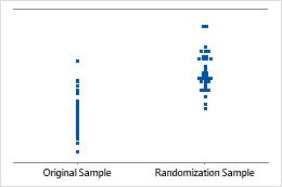
Individual value plot
An individual value plot displays the individual values in the sample. Each circle represents one observation. An individual value plot is especially useful when you have relatively few observations and when you also need to assess the effect of each observation.
Note
Minitab displays an individual value plot only when you take only one resample. Minitab displays both the original data and the resample data.
Interpretation
Minitab adjusts the data so that the center of the resamples is the same as the hypothesized mean. First, Minitab calculates the difference between the hypothesized mean and the mean of the original sample. Then Minitab adds or subtracts the difference to each value in the original sample. Resamples are taken from this adjusted data.
Sample mean equals hypothesized mean
Sample mean 2 standard deviations less than hypothesized mean
Null hypothesis and alternative hypothesis
- Null hypothesis
- The null hypothesis states that a population parameter (such as the mean, the standard deviation, and so on) is equal to a hypothesized value. The null hypothesis is often an initial claim that is based on previous analyses or specialized knowledge.
- Alternative hypothesis
- The alternative hypothesis states that a population parameter is smaller, greater, or different than the hypothesized value in the null hypothesis. The alternative hypothesis is what you might believe to be true or hope to prove true.
Interpretation
In the output, the null and alternative hypotheses help you to verify that you entered the correct value for the hypothesized mean.
Observed Sample
| Variable | N | Mean | StDev | Variance | Sum | Minimum | Median | Maximum |
|---|---|---|---|---|---|---|---|---|
| Time | 16 | 11.331 | 3.115 | 9.702 | 181.300 | 7.700 | 10.050 | 16.000 |
Randomization Test
| Null hypothesis | H₀: μ = 12 |
|---|---|
| Alternative hypothesis | H₁: μ < 12 |
| Number of Resamples | Mean | StDev | P-Value |
|---|---|---|---|
| 1000 | 11.9783 | 0.7625 | 0.199 |
In these results, the null hypothesis is that the population mean is equal to 12. The alternative hypothesis is that the mean is less than 12.
Number of Resamples
The number of resamples is the number of times Minitab takes a random sample with replacement from your original data set. Usually, a large number of resamples works best.
Minitab adjusts the data so that the center of the resamples is the same as the hypothesized mean. First, Minitab calculates the difference between the hypothesized mean and the mean of the original sample. Then Minitab adds or subtracts the difference to each value in the original sample. Resamples are taken from this adjusted data. The sample size for each resample is equal to the sample size of the original data set. The number of resamples equals the number of observations on the histogram.
Mean
The mean is the sum of all the means in the bootstrapping sample divided by the number of resamples. Minitab adjusts the data so that the center of the resamples is the same as the hypothesized mean.
Interpretation
Minitab displays two different mean values, the mean of the observed sample and the mean of the bootstrap distribution. The mean of the observed sample is an estimate of the population mean. The mean of the bootstrap distribution is usually close to the hypothesized mean. The larger the difference between these two values, the more evidence you would expect against the null hypothesis.
StDev (bootstrap sample)
The standard deviation is the most common measure of dispersion, or how spread out the data are about the mean. The symbol σ (sigma) is often used to represent the standard deviation of a population, while s is used to represent the standard deviation of a sample. Variation that is random or natural to a process is often referred to as noise. Because the standard deviation is in the same units as the data, it is usually easier to interpret than the variance.
The standard deviation of the bootstrap samples (also known as the bootstrap standard error) is an estimate of the standard deviation of the sampling distribution of the mean. Because the bootstrap standard error is the variation of sample means, whereas the standard deviation of the observed samples is the variation of individual observations, the bootstrap standard error is smaller.
Interpretation
Use the standard deviation to determine how spread out the means from the bootstrap sample are from the overall mean. A higher standard deviation value indicates greater spread in the means. A good rule of thumb for a normal distribution is that approximately 68% of the values fall within one standard deviation of the overall mean, 95% of the values fall within two standard deviations, and 99.7% of the values fall within three standard deviations.
Use the standard deviation of the bootstrap samples to estimate the precision of the bootstrap means. A smaller value indicates more precision. A larger standard deviation in the original sample usually results in a larger bootstrap standard error and a less powerful hypothesis test. A smaller sample size also usually results in a larger bootstrap standard error and a less powerful hypothesis test.
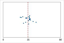
Hospital 1
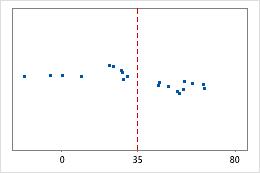
Hospital 2
Hospital discharge times
Administrators track the discharge time for patients who are treated in the emergency departments of two hospitals. Although the average discharge times are about the same (35 minutes), the standard deviations are significantly different. The standard deviation for hospital 1 is about 6. On average, a patient's discharge time deviates from the mean (dashed line) by about 6 minutes. The standard deviation for hospital 2 is about 20. On average, a patient's discharge time deviates from the mean (dashed line) by about 20 minutes.
P-Value
The p-value is the proportion of sample means that are as extreme as your original sample when you assume that the null hypothesis is true. A smaller p-value provides stronger evidence against the null hypothesis.
Interpretation
Use the p-value to determine whether the population mean is statistically different from the hypothesized mean.
- P-value ≤ α: The difference between the means is statistically significant (Reject H0)
- If the p-value is less than or equal to the significance level, the decision is to reject the null hypothesis. You can conclude that the difference between the population mean and the hypothesized mean is statistically significant. To calculate a confidence interval and determine whether the difference is practically significant, use Bootstrapping for 1-sample function. For more information, go to Statistical and practical significance.
- P-value > α: The difference between the means is not statistically significant (Fail to reject H0)
- If the p-value is greater than the significance level, the decision is to fail to reject the null hypothesis. You do not have enough evidence to conclude that the difference between the population mean and the hypothesized mean is statistically significant.