In This Topic
Step 1: Determine whether the regression line fits your data
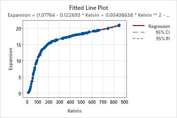
If your nonlinear model contains one predictor, Minitab displays the fitted line plot to show the relationship between the response and predictor data. The plot includes the regression line, which represents the regression equation. You can also choose to display the 95% confidence and prediction intervals on the plot.
- The sample contains an adequate number of observations throughout the entire range of all the predictor values.
- The model properly fits the curvature in the data. To determine which model is best, examine the plot, the standard error of the regression (S), and the Lack-of-Fit test when your data contain replicates.
- Look for any outliers, which can have a strong effect on the results. Try to identify the cause of any outliers. Correct any data entry or measurement errors. Consider removing data values that are associated with abnormal, one-time events (special causes). Then, repeat the analysis. For more information on detecting outliers, go to Unusual observations.
Step 2: Examine the relationship between the predictors and the response
Use the regression equation to describe the relationship between the response and the terms in the model. The regression equation is an algebraic representation of the regression line. Enter the value of each predictor into the equation to calculate the mean response value. Unlike linear regression, a nonlinear regression equation can take many forms.
For nonlinear equations, determining the effect that each predictor has on the response can be less intuitive than it is for linear equations. Unlike the parameter estimates in linear models, there is no consistent interpretation for the parameter estimates in nonlinear models. The correct interpretation for each parameter depends on the expectation function and the parameter's place in it. If your nonlinear model contains only one predictor, assess the fitted line plot to see the relationship between the predictor and response.
If you need to determine whether a parameter estimate is statistically significant, use the confidence intervals for the parameters. The parameter is statistically significant if the range excludes the null hypothesis value. Minitab cannot calculate p-values for parameters in nonlinear regression. For linear regression, the null hypothesis value for every parameter is zero, for no effect, and the p-value is based on this value. However, in nonlinear regression, the correct null hypothesis value for each parameter depends on the expectation function and the parameter's place in it.
For some data sets, expectation functions, and confidence levels, it is possible that one or both confidence bounds may not exist. Minitab indicates missing results with an asterisk. If the confidence interval has a missing bound, a lower confidence level might produce a two-sided interval.
Convergence on a solution does not necessarily guarantee that the model fit is optimal or that the sum of squared errors (SSE) are minimized. Convergence on incorrect parameter values can occur due to a local SSE minimum or an incorrect expectation function. Therefore, it is crucial to examine the parameter values, fitted line plot, and residual plots, to determine if the model fit and parameter values are reasonable.
Equation
3) / (1 - 0.00576099 * Kelvin + 0.000240537 * Kelvin ** 2 - 1.23144E-07 * Kelvin ** 3)
Key Result: Equation
In these results, there is one predictor and seven parameter estimates. The response variable is Expansion and the predictor variable is temperature on the Kelvin scale. The lengthy equation describes the relationship between the response and the predictors. The effect that a 1 degree Kelvin increase has on copper expansion highly depends on the starting temperature. The effect of changing temperatures on copper expansion cannot be easily summarized. Assess the fitted line plot to see the relationship between the predictor and response.
If you enter a value for temperature in Kelvin into the equation, the result is the fitted value for copper expansion.
Step 3: Determine how well the model fits your data
To determine how well the model fits your data, examine the statistics in the Model Summary table and the Lack of Fit table.
- S
-
Use S to assess how well the model describes the response.
S is measured in the units of the response variable and represents how far the data values fall from the fitted values. The lower the value of S, the better the model describes the response. However, a low S value by itself does not indicate that the model meets the model assumptions. You should check the residual plots to verify the assumptions.
- Lack of Fit
-
Minitab automatically displays the Lack of Fit table when your data contain replicates. Replicates are multiple observations with identical predictor values. If your data do not contain replicates, it is impossible to calculate the pure error that is required to perform this test. Different response values for replicates represent pure error because only random variation can cause differences between the observed response values.
To determine whether the model correctly specifies the relationship between the response and the predictors, compare the p-value for the lack-of-fit test to your significance level to assess the null hypothesis. The null hypothesis for the lack-of-fit test is that the model correctly specifies the relationship between the response and the predictors. Usually, a significance level (denoted as alpha or α) of 0.05 works well. A significance level of 0.05 indicates a 5% risk of concluding that the model does not correctly specify the relationship between the response and the predictors when the model does specify the correct relationship.- P-value ≤ α: The lack-of-fit is statistically significant
- If the p-value is less than or equal to the significance level, you conclude that the model does not correctly specify the relationship. To improve the model, you may need to add terms or transform your data.
- P-value > α: The lack-of-fit is not statistically significant
-
If the p-value is larger than the significance level, the test does not detect any lack-of-fit.
Lack of Fit
| Source | DF | SS | MS | F | P |
|---|---|---|---|---|---|
| Error | 229 | 1.53244 | 0.0066919 | ||
| Lack of Fit | 228 | 1.52583 | 0.0066922 | 1.01 | 0.679 |
| Pure Error | 1 | 0.00661 | 0.0066125 |
Summary
| Iterations | 15 |
|---|---|
| Final SSE | 1.53244 |
| DFE | 229 |
| MSE | 0.0066919 |
| S | 0.0818039 |
Key Results: S, Lack of Fit
In these results, S indicates that the standard deviation of the distance between the data values and the fitted values is approximately 0.08 units. The p-value for the lack-of-fit test is 0.679, which provides no evidence that the model fits the data poorly.
Step 4: Determine whether your model meets the assumptions of the analysis
Use the residual plots to help you determine whether the model is adequate and meets the assumptions of the analysis. If the assumptions are not met, the model may not fit the data well and you should use caution when you interpret the results.
For more information on how to handle patterns in the residual plots, go to Residual plots for Nonlinear Regression and click the name of the residual plot in the list at the top of the page.
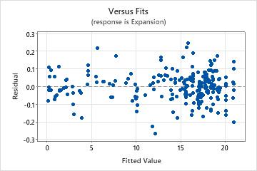
Residuals versus fits plot
Use the residuals versus fits plot to verify the assumption that the residuals are randomly distributed and have constant variance. Ideally, the points should fall randomly on both sides of 0, with no recognizable patterns in the points.
| Pattern | What the pattern may indicate |
|---|---|
| Fanning or uneven spreading of residuals across fitted values | Nonconstant variance |
| Curvilinear | A missing higher-order term |
| A point that is far away from zero | An outlier |
| A point that is far away from the other points in the x-direction | An influential point |
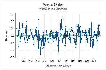
Residuals versus order plot
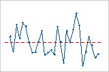
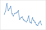
Trend
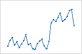
Shift
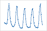
Cycle
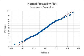
Normal probability plot of residuals
Use the normal probability plot of the residuals to verify the assumption that the residuals are normally distributed. The normal probability plot of the residuals should approximately follow a straight line.
| Pattern | What the pattern may indicate |
|---|---|
| Not a straight line | Nonnormality |
| A point that is far away from the line | An outlier |
| Changing slope | An unidentified variable |