Researchers in a food laboratory want to enhance a recipe for cheese fondue by improving the flavor, maximizing the amount that sticks to bread dipped into the fondue, and minimizing the amount that is burned at the bottom of the pot. The researchers design an extreme vertices mixture experiment to study the effects of the mixture blend and serving temperature.
To help visualize the design space for the extreme vertices experiment, the researchers create a simplex design plot.
- Open the sample data, FondueRecipe.MWX.
- Choose .
- Under Components, select Select a triplet of components for a single plot. Under X-Axis, choose Emmenthaler. Under Y-Axis, choose Gruyere. Under Z-Axis, choose Broth.
- Select Plot all level combinations.
- Click OK.
Interpret the results
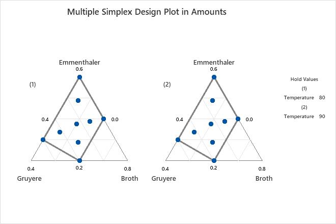
Minitab plots the design points on triangular axes. For more information, go to What the triangular coordinate system shows.
The simplex design plot shows that there are 18 points in the design space. The proportions of the components are selected for each point in such a manner that they sum to one. The solid grey contour represents the design space for this mixture design. In some designs, the plot can extend beyond the design space.
- Four vertex points that are at the corners of the grey constraint region.
- One center point in the center of the constraint region. This point corresponds to the blend in which the component proportions are the averages of the corresponding vertex proportions.
- Four axial points inside the constraint region. These points lie exactly halfway between the center point and a vertex.