In This Topic
Step 1: View the fit of the normal distribution
Use the normal probability plots to assess how closely the original and transformed data follow the normal distribution.
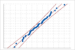
Good fit
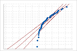
Poor fit
Note
If the original data are normally distributed, Minitab displays only a single probability plot and does not perform the Johnson transformation.
Step 2: Assess the fit of the normal distribution
Use the p-value to assess whether you can assume that the original and transformed data follow the normal distribution.
- A p-value that is less than alpha indicates that the normal distribution is not a good fit.
- A p-value that is greater than or equal to alpha indicates that there is not enough evidence of a poor distribution fit. You can assume the data follow the normal distribution.
If the Johnson transformation is effective, the p-value for the transformed data is greater than alpha.
Important
Use caution when you interpret results from a very small or a very large sample. If you have a very small sample, a goodness-of-fit test may not have enough power to detect significant deviations from the distribution. If you have a very large sample, the test may be so powerful that it detects even small deviations from the distribution that have no practical significance. Use the probability plots in addition to the p-values to evaluate the distribution fit.
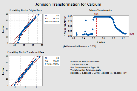
Key Result: P-Value
In these results, the p-value (0.046) for the original data is less than alpha (0.10), which indicates that the original calcium data are not normal. For the transformed data, the p-value (0.986) is greater than alpha. Therefore, you can assume that the transformed data follow a normal distribution.
Step 3: Examine the transformation function
Minitab displays the parameters of the Johnson transformation function that produces the best fit. Minitab uses this function to transform the original data.
For example, suppose the Johnson transformation function is 0.762475 + 0.870902 × Ln((X – 46.3174 ) / (59.6770 – X)). If the original data value for X is 50, then the transformed data value of 50 is calculated as 0.762475 + 0.870902 × Ln((50 – 46.3174) / (59.6770 – 50)), which equals –0.07893.
Note
To store all the transformed data values in the worksheet, enter a storage column when you perform the analysis.
For more information on the algorithm that Minitab uses to define the Johnson transformation function, go to Methods and formulas for transformations in Individual Distribution Identification and click "Methods and formulas for the Johnson Transformation".