N
The number of nonmissing values in the sample. N is the count of all the observed values.
| Total | N | N* |
|---|---|---|
| 149 | 141 | 8 |
Interpretation
Use N to assess your sample size.
Important
Use caution when you interpret results from a very small or a very large sample. If you have a very small sample, a goodness-of-fit test may not have enough power to detect significant deviations from the distribution. If you have a very large sample, the test may be so powerful that it detects even small deviations from the distribution that have no practical significance. Use the probability plots in addition to the p-values to evaluate the distribution fit.
N*
The number of missing values in the sample. N* is the count of the cells in the worksheet that contain the missing value symbol *.
| Total | N | N* |
|---|---|---|
| 149 | 141 | 8 |
Mean
The mean is calculated as the average of the data, which is the sum of all the observations divided by the number of observations.
Interpretation
Use the mean to describe the sample with a single value that represents the center of the data. Many statistical analyses use the mean as a standard reference point.
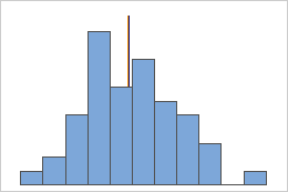
Mean and median in a symmetric distribution
Mean and median in a non-symmetric distribution
For the symmetric distribution, the mean (blue line) and median (orange line) are nearly the same. Therefore, the lines overlap and cannot be distinguished from one another. For the non-symmetric distribution, the data is skewed to the right, which causes the mean value to be greater than the median.
StDev
The standard deviation (StDev) is the most common measure of dispersion, or how spread out the data are about the mean. The symbol σ (sigma) is often used to represent the standard deviation of a population, and s is used to represent the standard deviation of a sample.
Interpretation
Use the standard deviation to determine how spread out the data are from the mean. A larger sample standard deviation indicates that your data are spread more widely around the mean.
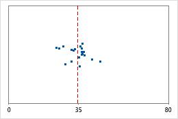
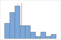
Hospital 1
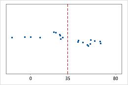
Hospital 2
Hospital discharge times
Administrators track the discharge time for patients who are treated in the emergency departments of two hospitals. Although the average discharge times are about the same (35 minutes), the standard deviations are significantly different. The standard deviation for hospital 1 is about 6. On average, a patient's discharge time deviates from the mean (dashed line) by about 6 minutes. The standard deviation for hospital 2 is about 20. On average, a patient's discharge time deviates from the mean (dashed line) by about 20 minutes.
Median
The median is the midpoint of the data set. This midpoint value is the point at which half of the observations are above the value and half of the observations are below the value. The median is determined by ranking the observations and finding the observation at the number [N + 1] / 2 in the ranked order. If the number of observations is even, the median is the value between the observations ranked at numbers N / 2 and [N / 2] + 1.
For this ordered data, the median is 13. That is, half of the values are less than or equal to 13, and half of the values are greater than or equal to 13.
Interpretation
Mean and median in a symmetric distribution
Mean and median in a non-symmetric distribution
For the symmetric distribution, the mean (blue line) and median (orange line) are nearly the same. Therefore, the lines overlap and cannot be distinguished from one another. For the non-symmetric distribution, the data is skewed to the right, which causes the mean value to be greater than the median.
Minimum
The smallest data value.
In these data, the minimum is 7.
| 13 | 17 | 18 | 19 | 12 | 10 | 7 | 9 | 14 |
Interpretation
Use the minimum to identify a possible outlier. If the value is unusually low, investigate its possible causes, such as a data-entry error or a measurement error.
One of the simplest ways to assess the spread of the data is to compare the minimum and maximum to determine its range. The range is the difference between the maximum and the minimum value in the data set. When you evaluate the spread of the data, also consider other measures, such as the standard deviation.
Maximum
The largest data value.
In these data, the maximum is 19.
| 13 | 17 | 18 | 19 | 12 | 10 | 7 | 9 | 14 |
Interpretation
Use the maximum to identify a possible outlier. If the value is unusually high, investigate its possible causes, such as a data-entry error or a measurement error.
One of the simplest ways to assess the spread of the data is to compare the minimum and maximum to determine its range. The range is the difference between the maximum and the minimum in the data set. When you evaluate the spread of the data, also consider other measures, such as the standard deviation.
Skewness
Skewness is the extent to which the data are not symmetrical.
Interpretation
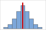
Figure A: Symmetrical, normally distributed data
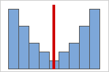
Figure B: Symmetrical, nonnormally distributed data
Symmetrical or non-skewed distributions
As data becomes more symmetrical, its skewness value approaches 0. Figure A shows normally distributed data, which by definition exhibits relatively little skewness. The line in middle of the histogram of normal data shows that the two sides mirror one another. Lack of skewness by itself, however, does not imply normality. Figure B shows a distribution where the two sides mirror one another, but the data is not normally distributed.
Positive- or right-skewed distributions
Positive-skewed data is also called right-skewed data because the "tail" of the distribution points to the right. Positive-skewed data has a skewness value that is greater than 0. Salary data often is positively skewed: many employees in a company make relatively low salaries while increasingly few people make very high salaries.
Negative- or left-skewed distributions
Negative-skewed data is often called left-skewed data because the "tail" of the distribution points to the left. Negative-skewed data has a skewness value that is less than 0. Failure rate data is often negatively skewed. For example, very few light bulbs burn out immediately, and most bulbs do not burn out for a long time.
Kurtosis
Kurtosis indicates how the tails of a distribution differ from the normal distribution.
Interpretation
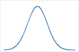
Baseline: Kurtosis value of 0
Data that follow a normal distribution perfectly have a kurtosis value of 0. Normally distributed data establish the baseline for kurtosis. Kurtosis that significantly deviates from 0 may indicate that the data are not normally distributed.
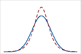
Positive kurtosis
A distribution that has a positive kurtosis value indicates that the distribution has heavier tails than the normal distribution. For example, data that follow a t-distribution have a positive kurtosis value. The solid line shows the normal distribution, and the dotted line shows a t-distribution with positive kurtosis.
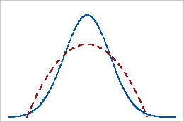
Negative kurtosis
A distribution that has a negative kurtosis value indicates that the distribution has lighter tails than the normal distribution. For example, data that follow a beta distribution with first and second shape parameters equal to 2 have a negative kurtosis value. The solid line shows the normal distribution and the dotted line shows a beta distribution with negative kurtosis.