Uses of the Weibull distribution to model reliability data
- What percentage of items are expected to fail during the burn-in period? For example, what percentage of fuses are expected to fail during the 8 hour burn-in period?
- How many warranty claims can be expected during the useful life phase? For example, how many warranty claims do you expect to receive during the 50,000-mile useful life of this tire?
- When is fast wear-out expected to occur? For example, when should maintenance be regularly scheduled to prevent engines from entering their wear-out phase?
The Weibull distribution can model data that are right-skewed, left-skewed, or symmetric. Therefore, the distribution is used to evaluate reliability across diverse applications, including vacuum tubes, capacitors, ball bearings, relays, and material strengths. The Weibull distribution can also model a hazard function that is decreasing, increasing or constant, allowing it to describe any phase of an item's lifetime.
The Weibull distribution may not work as effectively for product failures that are caused by chemical reactions or a degradation process like corrosion, which can occur with semiconductor failures. Usually, these types of situations are modeled using the lognormal distribution.
- Rayleigh distribution
- When the Weibull distribution has a shape parameter of 2, it is known as the Rayleigh distribution. This distribution is frequently used to describe measurement data in the field of communications engineering, such as measurements for input return loss, modulation side-band injection, carrier suppression, and RF fading. This distribution is also commonly used in the life testing of electrovacuum devices.
- Weakest link model
- The Weibull distribution can also model a life distribution with many identical and independent processes leading to failure, in which the first to get to a critical stage determines the time to failure. Extreme value theory serves as the basis for this "weakest link" model, where many flaws compete to be the eventual site of failure. Because the Weibull distribution can be theoretically derived from the smallest extreme value distribution, it can also provide an effective model for weakest-link applications such as capacitor, ball bearing, relay and material strength failures. However, if the variable of interest can take negative values, the smallest extreme value distribution is better, because the Weibull distribution can only model positive values due to its lower bound of 0.
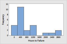
Example 1: Capacitors
Capacitors were tested at high stress to obtain failure data (in hours). The failure data were modeled by a Weibull distribution.
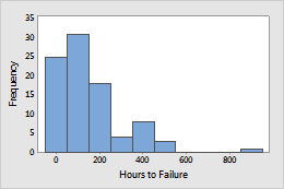
Example 2: Filaments
A light bulb company manufactures incandescent filaments that are not expected to wear out during an extended period of normal use. The engineers at the company want to guarantee the bulbs for 10 years of operation. Engineers stress the bulbs to simulate long-term use and record the hours until failure for each bulb.
Relationship between Weibull distribution parameters, reliability functions, and hazard functions
By adjusting the shape parameter, β, of the Weibull distribution, you can model the characteristics of many different life distributions.
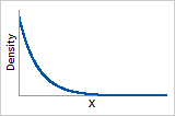
0 < ß < 1
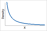
Probability density function
Exponentially decreasing from infinity
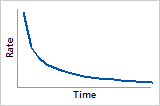
Hazard function
Initially high failure rate that decreases over time (first part of “bathtub” shaped hazard function)
ß = 1
Probability density function
Exponentially decreasing from 1/α (α = scale parameter)
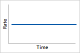
Hazard function
Constant failure rate during the life of the product (second part of "bathtub" shaped hazard function)
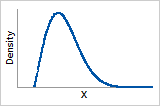
ß = 1.5
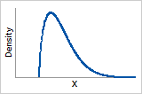
Probability density function
Increases to peak then decreases
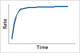
Hazard function
Increasing failure rate, with largest increase initially
ß = 2
Probability density function
Rayleigh distribution
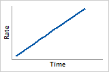
Hazard function
Linearly increasing failure rate
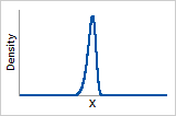
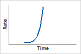
3 ≤ ß ≤4
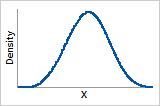
Probability density function
Bell-shaped
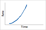
Hazard function
Increases quickly
ß > 10
Probability density function
Similar to extreme value distribution
Hazard function
Very quickly increasing