In This Topic
Anderson-Darling statistic (A2)
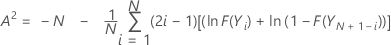
A2 measures the area between the fitted line (which is based on the chosen distribution) and the nonparametric step function (which is based on the plot points). The statistic is a squared distance that is weighted more heavily in the tails of the distribution. A small Anderson-Darling value indicates that the distribution fits the data better.
The Anderson-Darling normality test is defined as:
H0: The data follow a normal distribution
H1: The data do not follow a normal distribution
Formula
Notation
| Term | Description |
|---|---|
| F(Yi) |  , which is the cumulative distribution function of the standard normal distribution , which is the cumulative distribution function of the standard normal distribution |
| Yi | ordered data |
P-value for the Anderson-Darling normality test
A quantitative measure for reporting the result of the Anderson-Darling normality test is the p-value. A small p-value indicates that the null hypothesis is false.
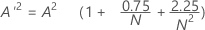
If you know A 2, you can calculate the p-value.
Let
- If 13 > A'2 > 0.600 then p = exp(1.2937 - 5.709 * A'2 + 0.0186(A'2)2)
- If 0.600 > A'2 > 0.340 then p = exp(0.9177 - 4.279 * A'2 – 1.38(A'2)2)
- If 0.340 > A'2 > 0.200 then p = 1 – exp(–8.318 + 42.796 * A'2 – 59.938(A'2)2)
- If A'2 < 0.200 then p = 1 – exp(–13.436 + 101.14 * A'2 – 223.73(A'2)2)
N nonmissing (N)
The number of non-missing values in the sample.
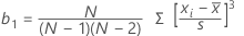
Standard deviation (StDev)
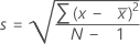
The sample standard deviation provides a measure of the spread of your data. It is equal to the square root of the sample variance.
Formula
 , then the standard deviation of the sample is:
Notation
| Term | Description |
|---|---|
| x i | i th observation |
 | mean of the observations |
| N | number of nonmissing observations |
Variance
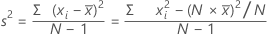
The variance measures how spread out the data are about their mean. The variance is equal to the standard deviation squared.
Formula
Notation
| Term | Description |
|---|---|
| xi | ith observation |
 | mean of the observations |
| N | number of nonmissing observations |
Skewness
Skewness is a measure of asymmetry. A negative value indicates skewness to the left, and a positive value indicates skewness to the right. A zero value does not necessarily indicate symmetry.
Formula
Notation
| Term | Description |
|---|---|
| xi | i th observation |
 | mean of the observations |
| N | number of nonmissing observations |
| s | standard deviation of the sample |
Kurtosis
Kurtosis is one measure of how different a distribution is from the normal distribution. A positive value usually indicates that the distribution has a sharper peak than the normal distribution. A negative value indicates that the distribution has a flatter peak than the normal distribution.
Formula

Notation
| Term | Description |
|---|---|
| xi | i th observation |
 | mean of the observations |
| N | number of nonmissing observations |
| s | standard deviation of the sample |
Mean
A commonly used measure of the center of a batch of numbers. The mean is also called the average. It is the sum of all observations divided by the number of (nonmissing) observations.
Formula

Notation
| Term | Description |
|---|---|
| xi | ith observation |
| N | number of nonmissing observations |
Minimum
The smallest value in your data set.
Maximum
The largest value in your data set.
1st quartile (Q1)
25% of your sample observations are less than or equal to the value of the 1st quartile. Therefore, the 1st quartile is also referred to as the 25th percentile.
Formula

Notation
| Term | Description |
|---|---|
| y | truncated integer value of w |
| w |  |
| z | fraction component of w that was truncated |
| xj | jth observation in the list of sample data, ordered from smallest to largest |
Note
When w is an integer, y = w, z = 0, and Q1 = xy.
Median
The sample median is in the middle of the data: at least half the observations are less than or equal to it, and at least half are greater than or equal to it.
Suppose you have a column that contains N values. To calculate the median, first order your data values from smallest to largest. If N is odd, the sample median is the value in the middle. If N is even, the sample median is the average of the two middle values.
For example, when N = 5 and you have data x1, x2, x3, x4, and x5, the median = x3.
When N = 6 and you have ordered data x1, x2, x3, x4, x5,and x6:
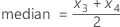
where x3 and x4 are the third and fourth observations.
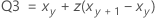
3rd quartile (Q3)
75% of your sample observations are less than or equal to the value of the third quartile. Therefore, the third quartile is also referred to as the 75th percentile.
Formula
Notation
| Term | Description |
|---|---|
| y | truncated value of w |
| w |
 |
| z | fraction component of w that was truncated away |
| xj | jth observation in the list of sample data, ordered from smallest to largest |
Note
When w is an integer, y = w, z = 0, and Q3 = xy.
Confidence interval for mean
Formula

Notation
| Term | Description |
|---|---|
 | mean |
| s | standard deviation of the sample |
| N | number nonmissing |
| t N, α | inverse cumulative probability of a t distribution with N – 1 degrees of freedom at 1 – α / 2; α = 1 – confidence level / 100 |
Confidence interval for the median
Minitab uses nonlinear interpolation to calculate the confidence interval for the true median 1. This method is a very good approximation for a wide variety of symmetric distributions including the normal distribution, the Cauchy distribution, and the uniform distribution. Examples of nonsymmetric distributions show adequate results that are always much more accurate than linear interpolation.
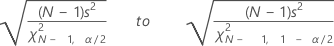
Confidence interval for the standard deviation
Minitab calculates a (1 – α) 100% confidence interval for the population standard deviation, σ. The confidence interval is very sensitive to the assumption that the data are normal. Even minor deviations from normality can result in a confidence interval that is misleading.
Formula
The confidence interval goes from:
Notation
| Term | Description |
|---|---|
| s | standard deviation |
| N | number nonmissing |
| χ2N, α | inverse cumulative probability of a χ2 with N degrees of freedom at 1 – α / 2; α = 1 – confidence level / 100 |