In This Topic
Estimated mean
Formula
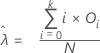
The mean for the Poisson distribution is estimated as:
Computation
| Data | 2 2 3 3 2 4 4 2 1 1 1 4 4 3 0 4 3 2 3 3 4 1 3 1 4 3 2 2 1 2 0 2 3 2 3 |
| Category (i) | Observed (Oi) | Estimated mean | Poisson probability (pi) |
|---|---|---|---|
| 0 | 2 | 0 * 2 = 0 | p0 = e-2.4 = 0.090718 |
| 1 | 6 | 1 * 6 = 6 | p1 = e-2.4 * 2.4 = 0.217723 |
| 2 | 10 | 2 * 10 = 20 | p2 = e-2.4 * (2.4)2/ 2! = 0.261268 |
| 3 | 10 | 3 * 10 = 30 | p3 = e-2.4 * (2.4)3/ 3! = 0.209014 |
 |
7 | 4 * 7 = 28 | p4 = 1 - (p0 + p1 +p2 + p3) = 0.221267 |
N = 35
Σ (i * Oi) = 84
Estimated Mean = 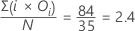
Notation
| Term | Description |
|---|---|
| N | sum of all observed values (O0 + O1 + ...+ Ok) |
| k | (the number of categories) - 1 |
| Oi | the observed number of events in the ith category |
| pi | Poisson probability |
Number of categories
Minitab determines categories using the following iterative methods:
Defining the first category
Let pi = P(X  xi )
xi )
Let i = 1: if N*pi  2, then the first category is defined as "
 x 1". If N*pi < 2, then increase i by one and repeat: if N*p 2
  2, then the first category is defined as "
 x 2". If N*pi < 2, increase i by one and repeat until N*pi
  2. Stop iterations either when this condition is first satisfied, or when xi is the third largest data value, and define the first category as "
 xi ". If the value of the first category is zero, then the first category is defined as "0" without the "less than or equal to" sign. The probability and expected value associated with the first category is pi and N*pi respectively. The observed value for the first category is the number of all data values
  xi .
xi .
Defining the last category
Conceptually, defining the last category is similar to defining the first category, but Minitab works backward starting from the largest data value.
The last category is " xj ", where xj is the largest data value greater than (1 + the data value of the first category), such that the category has an expected value greater than 2. The probability and expected value for the last category are pj and N*pj respectively, and the observed value is the number of data values
  xj .
xj .
Defining the middle categories
After determining the first and the last categories, Minitab determines the categories between them. Let "X  k" be the first category, and "X
  m" is the last category. If all integers between (k, m) have expected values
  2, then they all constitute a middle category. If not, Minitab uses a recursive loop to group multiple adjacent integers into categories with expected values
  2. There are some situations, such as a data set with few observations, where the expected value of a category will be less than 2.
Notation
| Term | Description |
|---|---|
| N | the total number of observations |
| xi | the i th value in the data set after sorting it from smallest to largest |
| pi | Poisson probability |
Poisson probability
Formula
The Poisson probability of the i th category (i < k) is,

The Poisson probability for the last category, where i = k,
pi = 1 – (p0 + p1 + ...+ pk-1)
Notation
| Term | Description |
|---|---|
| k | the number of categories |
| λ | the estimated mean from your sample |
Expected number
Formula
The expected number of observations in i th category is N * pi .
Notation
| Term | Description |
|---|---|
| N | sample size |
| pi | the Poisson probability associated with the i th category |
Contribution to chi-square
Formula
Contribution of the Ith category to the chi-square value is calculated as

Notation
| Term | Description |
|---|---|
| OI | the observed number of observations in the Ith category |
| EI | the expected number of observations in the Ith category |
Test statistic
Formula
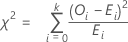
The chi-square goodness-of-fit test statistic is calculated as,
Notation
| Term | Description |
|---|---|
| k | (the number of categories) - 1 |
| Oi | the observed number of observations in the ith category |
| Ei | the expected number of observations in the ith category |
P-value and degrees of freedom
The p-value is:
Prob (X > Test statistic)
where X follows a chi-square distribution with k - 1 degrees of freedom if you use the MEAN subcommand, or k- 2 degrees of freedom if you do not use the MEAN subcommand.
Computation
| Data | 2 2 3 3 2 4 4 2 1 1 1 4 4 3 0 4 3 2 3 3 4 1 3 1 4 3 2 2 1 2 0 2 3 2 3 |
| Category (i) | Observed (Oi) | Estimated mean | Poisson probability (pi) |
|---|---|---|---|
| 0 | 2 | 0 * 2 = 0 | p0 = e -2.4 = 0.090718 |
| 1 | 6 | 1 * 6 = 6 | p1 = e -2.4 * 2.4 = 0.217723 |
| 2 | 10 | 2 * 10 = 20 | p2 = e -2.4 * (2.4)2/ 2! = 0.261268 |
| 3 | 10 | 3 * 10 = 30 | p3 = e -2.4 * (2.4)3/ 3! = 0.209014 |
 |
7 | 4 * 7 = 28 | p4 = 1 - (p0 + p1 +p2 + p3 ) = 0.221267 |
 = ( 0.434920 + 0.344527 + 0.080058 + 0.985114 + 0.071545) = 1.91622
k = 5= the number of categories
DF = 5- 2 = 3
p-value = P (X > 1.91622) = 0.590
Notation
| Term | Description |
|---|---|
| k | the number of categories |
| Oi | the observed number of observations in the ith category. |
| Ei | the expected number of observations in the ith category. |
 | chi-square goodness-of-fit test statistic |
| DF | degrees of freedom |