In This Topic
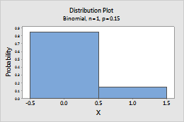
Bernoulli
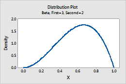
Beta
Complete the following steps to enter the parameters for the Beta distribution.
- In First shape parameter, enter a number that is greater than zero for the first shape parameter.
- In Second shape parameter, enter a number that is greater than zero for the second shape parameter.
For example, this plot shows a beta distribution that has a first shape of 3 and a second shape of 2.
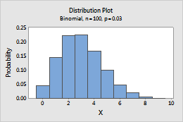
Binomial
Complete the following steps to enter the parameters for the Binomial distribution.
- In Number of trials, enter the sample size.
- In Event probability, enter a number between 0 and 1 for the probability that the outcome of interest occurs. An occurrence is called an "event".
For example, this plot shows a binomial distribution that has 100 trials and an event probability of 0.03.
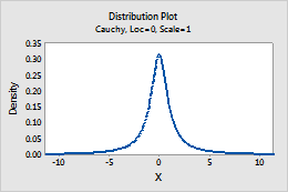
Cauchy
Complete the following steps to enter the parameters for the Cauchy distribution.
- In Location, enter a value that represents the location of the peak of the distribution.
- In Scale, enter a value that represents the spread of the distribution.
For example, this plot shows an Cauchy distribution that has a location of 0 and a scale of 1.
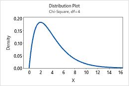
Chi-square
In Degrees of freedom, enter the number of degrees of freedom that define the Chi-square distribution.
For example, this plot shows a chi-square distribution that has 4 degrees of freedom.
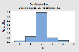
Discrete
Complete the following steps to enter the parameters for the Discrete distribution.
- In Values in, enter the column that contains the values to include in the distribution. Usually, the values are discrete events or counts that are represented by numeric values.
- In Probabilities in, enter the column that contains the probabilities for each value. Probabilities must be between 0 and 1, and must sum to 1.
In this worksheet, Value contains the counts to include in the distribution and Probability contains the probability of each count.
| C1 | C2 |
|---|---|
| Value | Probability |
| 0 | 0.03 |
| 1 | 0.13 |
| 2 | 0.70 |
| 3 | 0.10 |
| 4 | 0.04 |
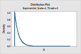
Exponential
Complete the following steps to enter the parameters for the Exponential distribution.
- In Scale, enter the scale parameter. The scale parameter equals the mean when the threshold parameter equals 0.
- In Threshold, enter the lower bound of the distribution.
For example, this plot shows an exponential distribution that has a scale of 1 and a threshold of 0.
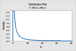
F
In Numerator degrees of freedom and Denominator degrees of freedom, enter the numerator and denominator degrees of freedom to define the F-distribution. For more information, go to F-distribution.
For example, this plot shows an F-distribution that has 1 numerator degrees of freedom and 1 denominator degrees of freedom.
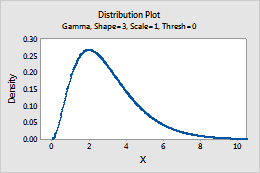
Gamma
Complete the following steps to enter the parameters for the Gamma distribution.
- In Shape parameter, enter the value that represents the shape of the distribution.
- In Scale parameter, enter the value that represents the scale of the distribution.
- In Threshold parameter, enter the lower bound of the distribution.
For example, this plot shows a gamma distribution that has a shape of 3, a scale of 1, and a threshold of 0.
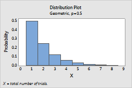
Geometric
Complete the following steps to enter the parameters for the Geometric distribution.
- In Event probability, enter a number between 0 and 1 for the probability of occurrence on each trial. An occurrence is called an "event".
- To specify which version of the geometric distribution to use, click Options, and select one of the following:
- Model the total number of trials: Model the total number of trials that are needed to produce one event.
- Model only the number of non-events: Model the number of nonevents that occur before one event occurs.
Tip
To change the default settings for future sessions of Minitab, choose .
For example, this plot shows a geometric distribution that models the total number of trials, and has an event probability of 0.5.
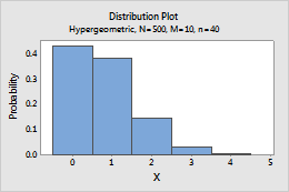
Hypergeometric
Complete the following steps to enter the parameters for the Hypergeometric distribution.
- In Population size (N), enter the total number of items in the population (N). When N is too large to be known, the binomial distribution approximates the hypergeometric distribution.
- In Event count in population (M), enter a number between 0 and N (population size) to represent the number of events in the population.
- In Sample size (n), enter the number of items that are sampled without replacement.
For example, this plot shows a hypergeometric distribution that has a population of 400, an event count of 10, and a sample size of 40.
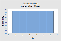
Integer
Complete the following steps to enter the parameters for the Integer distribution.
- In Minimum value, enter the lower end point of the distribution.
- In Maximum value, enter the upper end point of the distribution.
For example, this plot shows an integer distribution that has a minimum of 1 and a maximum of 6.
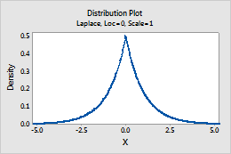
Laplace
Complete the following steps to enter the parameters for the Laplace distribution.
- In Location, enter a value that represents the location of the peak of the distribution.
- In Scale, enter a value that represents the spread of the distribution.
For example, this plot shows a Laplace distribution that has a location of 0 and a scale of 1.
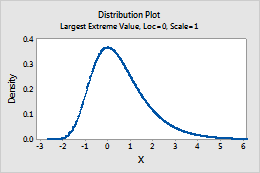
Largest extreme value
Complete the following steps to enter the parameters for the largest extreme value distribution. For more information, go to Smallest and largest extreme value distributions.
- In Location, enter a value that represents the location of the peak of the distribution.
- In Scale, enter a value that represents the spread of the distribution.
For example, this plot shows a largest extreme value distribution that has a location of 0 and a scale of 1.
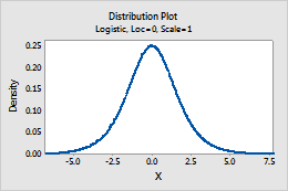
Logistic
Complete the following steps to enter the parameters for the Logistic distribution.
- In Location, enter a value that represents the location of the peak of the distribution.
- In Scale, enter a value that represents the spread of the distribution.
For example, this plot shows a logistic distribution that has a location of 0 and a scale of 1.
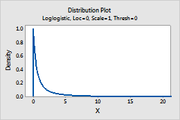
Loglogistic
Complete the following steps to enter the parameters for the Loglogistic distribution.
- In Location, enter a value that represents the location of the peak of the related logistic distribution.
- In Scale, enter a value that represents the spread of the related logistic distribution.
- In Threshold, enter the lower bound of the distribution.
For example, this plot shows a loglogistic distribution that has a location of 0, a scale of 1, and a threshold of 0.
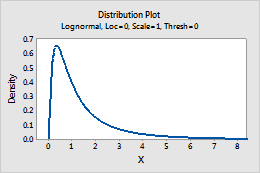
Lognormal
Complete the following steps to enter the parameters for the Lognormal distribution.
- In Location, enter a value that represents the location of the peak of the related normal distribution.
- In Scale, enter a value that represents the spread of the related normal distribution.
- In Threshold, enter the lower bound of the distribution.
For example, this plot shows a lognormal distribution that has a location of 0, a scale of 1, and a threshold of 0.
Multivariate normal
Complete the following steps to enter the parameters for the Multivariate normal distribution.
- In Mean column, enter the column that contains the vector of means.
- In Variance-Covariance matrix, enter the matrix (for example, M1) that contains the variances and covariances of the variables in the same order as in the mean column.
In this example, the data are from three correlated, normal random variables. The means are in C1, and the variance-covariance matrix is in columns C2–C4.
| C1 | C2 | C3 | C4 |
|---|---|---|---|
| 2.0 | 13.0321 | 2.6544 | 0.0899 |
| 100.1 | 2.6544 | 6.5883 | 1.4438 |
| 151.3 | 0.0899 | 1.4438 | 12.2219 |
- Choose .
- In Copy from columns, enter C2-C4.
- In Store Copied Data, under In current worksheet, in matrix:, enter M1.
- Click OK.
Now, you can generate random data from the multivariate normal distribution.
- Choose .
- In Number of rows of data to generate, enter the number of rows that you want. For this example, enter 18.
- In Store in column(s), enter your storage columns. For this example, enter C6-C8.
- In Mean column, enter the column that contains the means. For this example, enter C1.
- In Variance-Covariance matrix, enter the matrix. For this example, enter M1.
- Click OK.
Tip
To get the same sample as in the table below, set the random generator base before you generate the random sample. Choose and enter 5.
| C6 | C7 | C8 |
|---|---|---|
| 1.61033 | 99.192 | 148.814 |
| 0.45883 | 96.093 | 144.679 |
| −0.46745 | 101.041 | 148.936 |
| … | … | … |
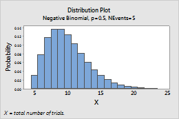
Negative binomial
Complete the following steps to enter the parameters for the Negative binomial distribution.
- In Event probability, enter a number between 0 and 1 for the probability of occurrence on each trial. An occurrence is called an "event".
- In Number of events needed, enter a positive integer that represents the number of times the event must occur.
- To specify which version of the negative binomial distribution to use, click Options, and select one of the following:
- Model the total number of trials: Model the total number of trials that are needed to produce the specified number of events.
- Model only the number of non-events: Model the number of nonevents that occur before the specified number of events occur.
Tip
To change the default settings for future sessions of Minitab, choose .
For example, this plot shows a negative binomial distribution that models the total number of trials, and has an event probability of 0.5 and 5 events.
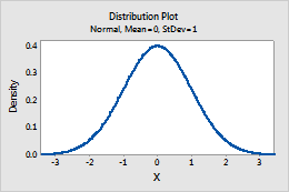
Normal
Complete the following steps to enter the parameters for the Normal distribution.
- In Mean, enter the value for the center of the distribution.
- In Standard deviation, enter the value for the spread of the distribution.
For example, this plot shows a normal distribution that has a mean of 0 and a standard deviation of 1.
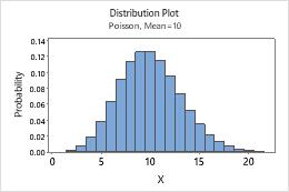
Poisson
In Mean, enter the value for the average rate of occurrence. For more information, go to Poisson distribution.
For example, this plot shows a Poisson distribution that has a mean of 10.
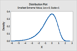
Smallest extreme value
Complete the following steps to enter the parameters for the smallest extreme value distribution. For more information, go to Smallest and largest extreme value distributions.
- In Location, enter a value that represents the location of the peak of the distribution.
- In Scale, enter a value that represents the spread of the distribution.
For example, this plot shows a smallest extreme value distribution that has a location of 0 and a scale of 1.
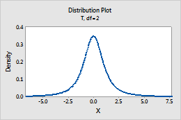
t
In Degrees of freedom, enter the degrees of freedom to define the t-distribution. For more information, go to t-distribution.
For example, this plot shows a t-distribution that has 2 degrees of freedom.
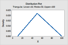
Triangular
Complete the following steps to enter the parameters for the Triangular distribution.
- In Lower endpoint, enter the minimum value for the distribution.
- In Mode, enter the value for the peak of the distribution.
- In Upper endpoint, enter the maximum value for the distribution.
For example, this plot shows a triangular distribution that has a lower end point of 10, a mode of 50, and an upper end point of 100.
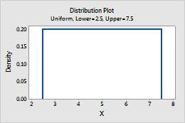
Uniform
Complete the following steps to enter the parameters for the Uniform distribution.
- In Lower endpoint, enter the minimum value for the distribution.
- In Upper endpoint, enter the maximum value for the distribution.
For example, this plot shows a uniform distribution that has a lower endpoint of 2.5 and an upper endpoint of 7.5.
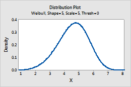
Weibull
Complete the following steps to enter the parameters for the Weibull distribution.
- In Shape parameter, enter the value that represents the shape of the distribution.
- In Scale parameter, enter the value that represents the scale of the distribution.
- In Threshold parameter, enter the lower bound of the distribution.
For example, this plot shows a Weibull distribution that has a location of 5, a scale of 5, and a threshold of 0.