In This Topic
N
The sample size (N) is the number of complete data points for a pair of variables. Any row with missing data for either one of a pair of variables does not count towards the sample size.
| C1 | C2 | |
|---|---|---|
| A | B | |
| 1 | 18 | 2 |
| 2 | 17 | 20 |
| 3 | 12 | 16 |
| 4 | 19 | 22 |
| 5 | 15 | 32 |
| 6 | 6 | 25 |
| C1 | C2 | |
|---|---|---|
| A | B | |
| 1 | 18 | 18 |
| 2 | 17 | 28 |
| 3 | 12 | * |
| 4 | 19 | 8 |
| 5 | 15 | 19 |
| 6 | 6 | 25 |
| C1 | C2 | |
|---|---|---|
| A | B | |
| 1 | 18 | 9 |
| 2 | 28 | 5 |
| 3 | * | * |
| 4 | 8 | 23 |
| 5 | 19 | 11 |
| 6 | 25 | 25 |
| C1 | C2 | |
|---|---|---|
| A | B | |
| 1 | 18 | 20 |
| 2 | 28 | * |
| 3 | * | 9 |
| 4 | 8 | 3 |
| 5 | 19 | * |
| 6 | * | 3 |
Pearson Correlations
The correlation matrix shows the correlation values, which measure the degree of linear relationship between each pair of variables. The correlation values can fall between -1 and +1. If the two variables tend to increase and decrease together, the correlation value is positive. If one variable increases while the other variable decreases, the correlation value is negative.
Interpretation
Use the correlation matrix to assess the strength and direction of the relationship between two variables. A high, positive correlation values indicates that the variables measure the same characteristic. If the items are not highly correlated, then the items may measure different characteristics or may not be clearly defined.
Correlations
| Age | Residence | Employ | Savings | Debt | |
|---|---|---|---|---|---|
| Residence | 0.838 | ||||
| Employ | 0.848 | 0.952 | |||
| Savings | 0.552 | 0.570 | 0.539 | ||
| Debt | 0.032 | 0.186 | 0.247 | -0.393 | |
| Credit cards | -0.130 | 0.053 | 0.023 | -0.410 | 0.474 |
- Residence and Age, 0.838
- Employ and Age, 0.848
- Employ and Residence, 0.952
- Debt and Savings , −0.393
- Credit cards and Age, −0.130
- Credit cards and Savings, −0.410
Spearman Correlations
Use the Spearman correlation coefficient to examine the strength and direction of the monotonic relationship between two continuous or ordinal variables. In a monotonic relationship, the variables tend to move in the same relative direction, but not necessarily at a constant rate. To calculate the Spearman correlation, Minitab ranks the raw data. Then, Minitab calculates the correlation coefficient on the ranked data.
- Strength
-
The correlation coefficient can range in value from −1 to +1. The larger the absolute value of the coefficient, the stronger the relationship between the variables.
For the Spearman correlation, an absolute value of 1 indicates that the rank-ordered data are perfectly linear. For example, a Spearman correlation of −1 means that the highest value for Variable A is associated with the lowest value for Variable B, the second highest value for Variable A is associated with the second lowest value for Variable B, and so on.
- Direction
-
The sign of the coefficient indicates the direction of the relationship. If both variables tend to increase or decrease together, the coefficient is positive, and the line that represents the correlation slopes upward. If one variable tends to increase as the other decreases, the coefficient is negative, and the line that represents the correlation slopes downward.
The following plots show data with specific Spearman correlation coefficient values to illustrate different patterns in the strength and direction of the relationships between variables.
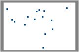
No relationship: Spearman rho = 0
The points fall randomly on the plot, which indicates that there is no relationship between the variables.
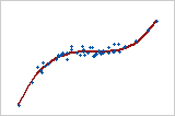
Strong positive relationship: Spearman rho = 0.948
The points fall close to the line, which indicates that there is a strong relationship between the variables. The relationship is positive because the variables increase concurrently.
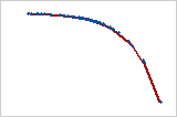
Strong negative relationship: Spearman rho = 1.0
The points fall close to the line, which indicates that there is a strong relationship between the variables. The relationship is negative because as one variable increases, the other variable decreases.
It is never appropriate to conclude that changes in one variable cause changes in another based on correlation alone. Only properly controlled experiments enable you to determine whether a relationship is causal.
Interpretation
Correlations
| Age | Residence | Employ | Savings | Debt | |
|---|---|---|---|---|---|
| Residence | 0.824 | ||||
| Employ | 0.830 | 0.912 | |||
| Savings | 0.570 | 0.571 | 0.496 | ||
| Debt | -0.198 | -0.142 | -0.056 | -0.605 | |
| Credit cards | -0.179 | 0.069 | 0.036 | -0.480 | 0.353 |
Pairwise Spearman Correlations
| Sample 1 | Sample 2 | N | Correlation | 95% CI for ρ | P-Value |
|---|---|---|---|---|---|
| Residence | Age | 30 | 0.824 | (0.624, 0.922) | 0.000 |
| Employ | Age | 30 | 0.830 | (0.636, 0.926) | 0.000 |
| Savings | Age | 30 | 0.570 | (0.236, 0.783) | 0.001 |
| Debt | Age | 30 | -0.198 | (-0.524, 0.178) | 0.293 |
| Credit cards | Age | 30 | -0.179 | (-0.508, 0.197) | 0.345 |
| Employ | Residence | 30 | 0.912 | (0.798, 0.963) | 0.000 |
| Savings | Residence | 30 | 0.571 | (0.237, 0.784) | 0.001 |
| Debt | Residence | 30 | -0.142 | (-0.479, 0.232) | 0.454 |
| Credit cards | Residence | 30 | 0.069 | (-0.300, 0.419) | 0.719 |
| Savings | Employ | 30 | 0.496 | (0.144, 0.737) | 0.005 |
| Debt | Employ | 30 | -0.056 | (-0.408, 0.311) | 0.768 |
| Credit cards | Employ | 30 | 0.036 | (-0.328, 0.392) | 0.849 |
| Debt | Savings | 30 | -0.605 | (-0.804, -0.283) | 0.000 |
| Credit cards | Savings | 30 | -0.480 | (-0.726, -0.124) | 0.007 |
| Credit cards | Debt | 30 | 0.353 | (-0.020, 0.639) | 0.056 |
In these results, the Spearman correlation between Residence and Age is 0.824, which indicates that there is a positive relationship between the variables. The confidence interval for rho is from 0.624 to 0.922. The p-value is 0.000, which indicates that the relationship is statistically significant at the α = 0.05 level.
The Spearman correlation between Debt and Savings is -0.605 and between Credit cards and Savings is -0.480. The relationship between these variables is negative, which indicates that as Debt and Credit cards increase, Savings decreases.
Rows used
When the data have no missing values, the number of rows used is the same as the number of rows with data. When the data have missing values, the number can be a range. The least number in the range is the number of rows used for the pairs of columns with the fewest complete pairs of data points. The greatest number in the range is the number of rows used for the pairs of columns with the most complete pairs of data points. To see the number of rows for each pair of columns, display the Pairwise correlation table.
Confidence Intervals for Correlation
The confidence interval provides a range of likely values for the correlation coefficients. Because samples are random, two samples from a population are unlikely to yield identical confidence intervals. But, if you repeated your sample many times, a certain percentage of the resulting confidence intervals or bounds would contain the unknown correlation coefficient. The percentage of these confidence intervals or bounds that contain the correlation coefficient is the confidence level of the interval.
For example, a 95% confidence level indicates that if you take 100 random samples from the population, you could expect approximately 95 of the samples to produce intervals that contain the correlation coefficient.
An upper bound defines a value that the population difference is likely to be less than. A lower bound defines a value that the population difference is likely to be greater than.
The confidence intervals for the Pearson correlation are sensitive to the normality of the underlying bivariate distribution. If the data deviate from normality, then the confidence intervals may be inaccurate regardless of the magnitude of the sample size.
The confidence intervals for Spearman correlations are based on ranks and are less sensitive to the underlying bivariate distribution assumption.
Interpretation
The confidence interval helps you assess the practical significance of your results. Use your specialized knowledge to determine whether the confidence interval includes values that have practical significance for your situation. If the interval is too wide to be useful, consider increasing your sample size. For more information, go to Ways to get a more precise confidence interval.
Pairwise Pearson Correlations
| Sample 1 | Sample 2 | N | Correlation | 95% CI for ρ | P-Value |
|---|---|---|---|---|---|
| Residence | Age | 30 | 0.838 | (0.684, 0.920) | 0.000 |
| Employ | Age | 30 | 0.848 | (0.702, 0.926) | 0.000 |
| Savings | Age | 30 | 0.552 | (0.240, 0.761) | 0.002 |
| Debt | Age | 30 | 0.032 | (-0.332, 0.388) | 0.865 |
| Credit cards | Age | 30 | -0.130 | (-0.468, 0.242) | 0.494 |
| Employ | Residence | 30 | 0.952 | (0.901, 0.977) | 0.000 |
| Savings | Residence | 30 | 0.570 | (0.264, 0.772) | 0.001 |
| Debt | Residence | 30 | 0.186 | (-0.187, 0.512) | 0.326 |
| Credit cards | Residence | 30 | 0.053 | (-0.313, 0.406) | 0.779 |
| Savings | Employ | 30 | 0.539 | (0.222, 0.753) | 0.002 |
| Debt | Employ | 30 | 0.247 | (-0.125, 0.557) | 0.189 |
| Credit cards | Employ | 30 | 0.023 | (-0.340, 0.380) | 0.906 |
| Debt | Savings | 30 | -0.393 | (-0.660, -0.038) | 0.032 |
| Credit cards | Savings | 30 | -0.410 | (-0.671, -0.059) | 0.024 |
| Credit cards | Debt | 30 | 0.474 | (0.138, 0.713) | 0.008 |
In these results, Residence and Age have a positive linear correlation of 0.838. You can be 95% confident that the population correlation coefficient is between 0.684 and 0.920. Usually, when the correlation is stronger, the confidence interval is narrower. For instance, Credit cards and Age have a weak correlation and the 95% confidence interval ranges from -0.468 to 0.242.
P-Value
The p-value is a probability that measures the evidence against the null hypothesis. A smaller p-value provides stronger evidence against the null hypothesis.
Interpretation
Use the p-value to determine whether the correlation coefficient is statistically significant.
- P-value ≤ α: The correlation is statistically significantly (Reject H0)
- If the p-value is less than or equal to the significance level, the decision is to reject the null hypothesis. You can conclude that the correlation is statistically significant. Use your specialized knowledge to determine whether the difference is practically significant. For more information, go to Statistical and practical significance.
- P-value > α: The correlation is not statistically significant (Fail to reject H0)
- If the p-value is greater than the significance level, the decision is to fail to reject the null hypothesis. You do not have enough evidence to conclude that the correlation is statistically significant.
The p-value procedures for both Pearson correlation and Spearman correlation are robust to departures from normality. The p-values are usually accurate for n ≥ 25, regardless of the parent population of the sample.
Pairwise Pearson Correlations
| Sample 1 | Sample 2 | N | Correlation | 95% CI for ρ | P-Value |
|---|---|---|---|---|---|
| Residence | Age | 30 | 0.838 | (0.684, 0.920) | 0.000 |
| Employ | Age | 30 | 0.848 | (0.702, 0.926) | 0.000 |
| Savings | Age | 30 | 0.552 | (0.240, 0.761) | 0.002 |
| Debt | Age | 30 | 0.032 | (-0.332, 0.388) | 0.865 |
| Credit cards | Age | 30 | -0.130 | (-0.468, 0.242) | 0.494 |
| Employ | Residence | 30 | 0.952 | (0.901, 0.977) | 0.000 |
| Savings | Residence | 30 | 0.570 | (0.264, 0.772) | 0.001 |
| Debt | Residence | 30 | 0.186 | (-0.187, 0.512) | 0.326 |
| Credit cards | Residence | 30 | 0.053 | (-0.313, 0.406) | 0.779 |
| Savings | Employ | 30 | 0.539 | (0.222, 0.753) | 0.002 |
| Debt | Employ | 30 | 0.247 | (-0.125, 0.557) | 0.189 |
| Credit cards | Employ | 30 | 0.023 | (-0.340, 0.380) | 0.906 |
| Debt | Savings | 30 | -0.393 | (-0.660, -0.038) | 0.032 |
| Credit cards | Savings | 30 | -0.410 | (-0.671, -0.059) | 0.024 |
| Credit cards | Debt | 30 | 0.474 | (0.138, 0.713) | 0.008 |
In these results, there are many p-values that are less than the significance level of 0.05, which indicates that the Pearson correlation coefficients are statistically significant.
Note
There are cases where because of extreme data points, the p-value might be small, but the confidence interval is very wide. For instance, with Credit cards and Debt, the 95% CI is very wide, but the p-value is small. When you examine the matric plot, you can see an extreme data point.
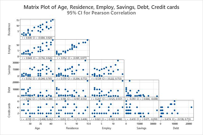
Matrix Plot
The matrix plot is an array of scatterplots. Each scatterplot in the matrix graphs the scores for a pair of items on the x and y axes.
Interpretation
Use the plot to visually assess the relationship between every combination of variables. The relationships can be linear, monotonic, or neither. Also use the matrix plot to look for outliers that can heavily influence the results. For more information on the types of relationships, go to Linear, nonlinear, and monotonic relationships.
This matrix plot suggests that all pairs of items have a positive linear relationship.