Interpret the key results for Orthogonal Regression

Complete the following steps to interpret an orthogonal regression analysis. Key output includes the confidence intervals for the coefficients, the fitted line plot, and the residual plots.

In This Topic

Step 1: Determine whether the measurements from two instruments or methods differ
Step 2: Determine whether the regression line fits your data

Step 1: Determine whether the measurements from two instruments or methods differ

You often use orthogonal regression in clinical chemistry or a laboratory to determine whether two instruments or methods provide comparable measurements. If the confidence interval for the constant term contains zero and the interval for the linear term contains 1, then you can usually conclude that the measurements from the two instruments are comparable.

You should also examine the plot with the fitted line to determine how well the model fits the data.

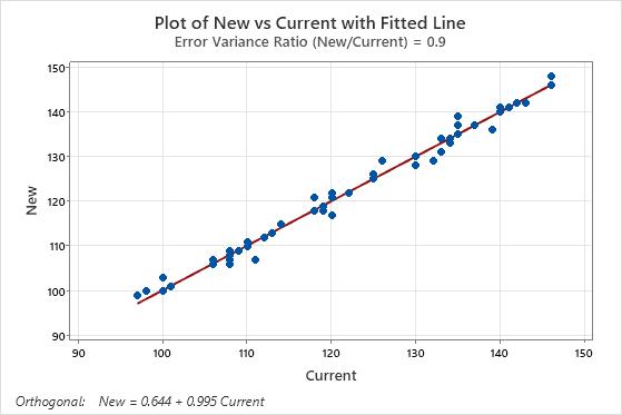
Error Variance Ratio (New/Current): 0.9

Regression Equation
New = 0.644 + 0.995 Current

Coefficients

Predictor	Coef	SE Coef	Z	P	Approx 95% CI
Constant	0.64441	1.74470	0.3694	0.712	(-2.77513, 4.06395)
Current	0.99542	0.01415	70.3461	0.000	(0.96769, 1.02315)

Error Variances

Variable	Variance
New	1.07856
Current	1.19840

Key Result: Approx 95% CI

In these results, the confidence interval for the constant term is approximately (−3, 4). Because the interval contains 0, this part of the analysis does not provide evidence that the measurements from the two instruments differ.

The confidence interval for the linear term is approximately (0.97, 1.02). Because the interval contains 1, this part of the analysis does not provide evidence that the measurements from the two instruments differ.

Because neither interval provides evidence that the measurements from the two instruments differ, you usually conclude that the measurements are comparable. You should also verify that the model fits the data well by examining the plot with the fitted line and the residual plots.

Step 2: Determine whether the regression line fits your data

Use the plot and the fitted line to assess whether the orthogonal regression equation is a good fit for the data. When the model fits the data, the points fall closely to the regression line. In particular, you can examine the fitted line plot for these criteria:

The sample contains an adequate number of observations throughout the entire range of all predictor values.
The sample contains no curvature that the model does not fit.
The sample contains no outliers, which can have a strong effect on the results. Try to identify the cause of any outliers. Correct any data entry or discernible measurement errors. Consider removing data values that are associated with abnormal, one-time events (special causes). Then, repeat the analysis.

This plot shows an example of measurements from two instruments or methods that are comparable. The points follow the fitted line with minimal scatter and without any pattern that reveals systematic differences between the methods.

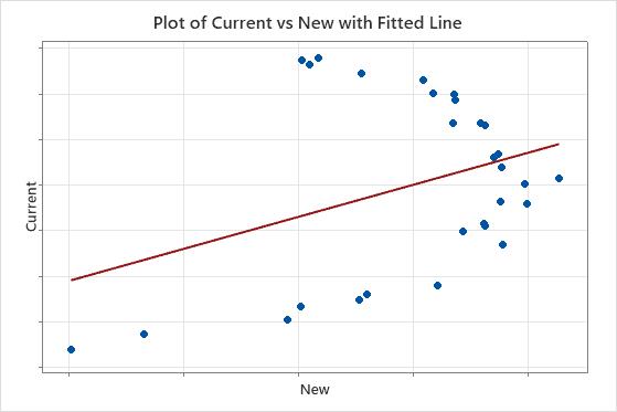
In the results below, the confidence intervals for the coefficients do not provide evidence that the measurements of the two instruments differ. However, the plot shows that points do not fall close to the line, which indicates that the measurements from the two instruments are not comparable. Because the data do not fit the equation, the usual conclusion is that the instruments differ.

Coefficients

Predictor	Coef	SE Coef	Z	P	Approx 95% CI
Constant	-0.00000	0.215424	-0.0000	1.000	(-0.422224, 0.42222)
New	1.00000	0.517586	1.9320	0.053	(-0.014450, 2.01445)